Ai Overview
Real estate token liquidity pool mechanics in 2026 leverage automated market makers (AMMs) to solve the thin-market problem inherent in fractional property ownership. Imagine a liquidity provider deposits 100 property tokens worth $100 each and 10,000 USDC into a pool, creating a 50-50 value split ($10,000 each side). If the property token price doubles to $200, arbitrage traders will buy cheap tokens from the pool until the price matches external markets. The provider’s share is now worth about $28,284 total (70.
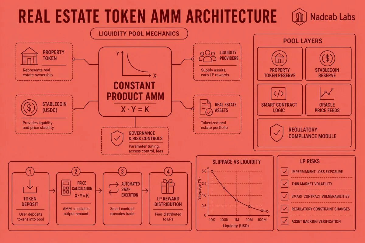
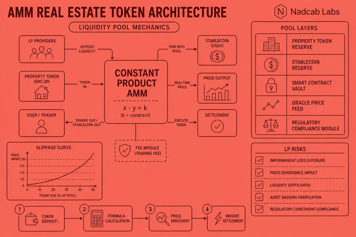
Real estate token liquidity pool mechanics in 2026 leverage automated market makers (AMMs) to solve the thin-market problem inherent in fractional property ownership. Unlike traditional order-book exchanges, AMMs use mathematical formulas—primarily the constant product model (x·y=k)—to enable instant, permissionless trading of property tokens against stablecoins or other digital assets. This architecture transforms illiquid real estate into tradable digital securities while introducing new dynamics like impermanent loss, slippage, and liquidity provider incentives that differ fundamentally from standard crypto token pools due to the underlying asset backing and regulatory constraints.
Key Takeaways
- AMMs replace order books for property tokens, using constant product formulas to enable 24/7 trading even with thin markets.
- Impermanent loss affects liquidity providers when real estate token prices diverge from paired assets, requiring stable swap curves or single-sided staking for mitigation.
- Slippage increases exponentially with trade size in shallow pools; institutional buyers need deep liquidity or concentrated liquidity models.
- Liquidity providers earn trading fees, yield farming rewards, and protocol tokens but face unique risks from low-volatility property assets.
- Stable swap variants and layer 2 implementations optimize capital efficiency and reduce transaction costs for tokenized real estate.
- Pool depth directly impacts price discovery quality and investor confidence in property token markets.
How Do Automated Market Makers Enable Real Estate Token Trading in 2026?
Automated market makers fundamentally change how fractional property ownership trades by replacing the traditional order-book model with algorithmic liquidity pools. In conventional exchanges, buyers and sellers submit limit orders that sit idle until matched—a system that fails when dealing with illiquid assets like tokenized real estate where trading volume is inherently low. AMMs solve this by maintaining reserves of two tokens in a pool and using a mathematical formula to determine prices automatically.
The constant product formula (x·y=k) is the foundation of most Real Estate Tokenization liquidity pools. Here, x represents the quantity of real estate tokens in the pool, y represents the paired asset (typically a stablecoin like USDC), and k is a constant. When someone buys property tokens from the pool, they deposit stablecoins (increasing y) and withdraw property tokens (decreasing x), but the product x·y must always equal k. This creates an automatic pricing curve where the price moves based on the ratio of assets in the pool.
For example, if a pool holds 10,000 property tokens and 1,000,000 USDC, the constant k equals 10,000,000,000. If a buyer wants 100 property tokens, they must deposit enough USDC to maintain that constant after the trade. The formula calculates the exact amount: the new x would be 9,900 tokens, so the new y must be 1,010,101 USDC (since 9,900 × 1,010,101 ≈ 10,000,000,000). The buyer pays 10,101 USDC for 100 tokens, an effective price of roughly 101 USDC per token—higher than the initial 100 USDC per token ratio due to slippage.
This mechanism works continuously without waiting for counterparties. Every trade instantly rebalances the pool and adjusts the price, making markets for property tokens that would otherwise sit dormant for days or weeks. The approach is particularly valuable for Financial Services platforms that need to offer investors exit liquidity without maintaining expensive market-making operations or relying on sporadic peer-to-peer matches.
| Exchange Model | Liquidity Source | Price Discovery | Minimum Liquidity | Best for Property Tokens |
|---|---|---|---|---|
| Order Book | Individual traders | Bid-ask spread | High (many active traders) | No (illiquid markets fail) |
| Constant Product AMM | Pooled capital | Algorithmic curve | Medium (2 assets locked) | Yes (instant trades) |
| Stable Swap AMM | Pooled capital | Flat curve near peg | Low (efficient capital use) | Ideal (low volatility assets) |
| Concentrated Liquidity | Pooled capital (range-bound) | Custom price ranges | Very low (capital efficient) | Yes (predictable price ranges) |
The thin-market problem is endemic to real estate because properties are unique, high-value, and infrequently traded. Even after tokenization, a single apartment building might generate only a few trades per week. Traditional exchanges would show wide bid-ask spreads or no bids at all during off-hours. AMMs guarantee that a buyer can always execute a trade at a calculable price, even at 3 AM on a Sunday, because the pool itself is the counterparty. This 24/7 liquidity is critical for institutional investors who need predictable exit strategies and for retail investors who expect the same instant execution they get with stocks or standard crypto tokens.
What Is Impermanent Loss and Why Does It Matter for Property Token Liquidity Providers in 2026?
Impermanent loss is the hidden cost liquidity providers face when the relative prices of pooled assets change. In a real estate token pool paired with a stablecoin, if the property token appreciates significantly while the stablecoin remains at $1, the AMM formula automatically rebalances the pool by selling property tokens and accumulating more stablecoins. The liquidity provider ends up with fewer high-value property tokens and more low-value stablecoins than if they had simply held both assets separately. This loss is “impermanent” because it only becomes permanent when the provider withdraws their liquidity; if prices revert, the loss disappears.
The mathematical mechanism is straightforward. Imagine a liquidity provider deposits 100 property tokens worth $100 each and 10,000 USDC into a pool, creating a 50-50 value split ($10,000 each side). The constant k equals 100 × 10,000 = 1,000,000. If the property token price doubles to $200, arbitrage traders will buy cheap tokens from the pool until the price matches external markets. The new equilibrium occurs when the pool holds approximately 70.7 property tokens and 14,142 USDC (since 70.7 × 14,142 ≈ 1,000,000). The provider’s share is now worth about $28,284 total (70.7 tokens × $200 + 14,142 USDC). If they had held the original 100 tokens and 10,000 USDC separately, they would have $30,000 (100 × $200 + 10,000). The impermanent loss is $1,716, or about 5.7%.
For Real Estate Tokenization Models, impermanent loss presents unique challenges because property valuations typically move slowly and predictably compared to volatile crypto assets. A tokenized office building might appreciate 3-5% annually, while its paired stablecoin remains flat. This low volatility reduces impermanent loss risk significantly. However, sudden market shocks—like a major tenant bankruptcy or interest rate spike—can cause sharp price movements that trigger substantial rebalancing losses before the property’s fundamental value recovers.
Real-world scenarios illustrate the risk spectrum. In a stable market where a residential property token appreciates 2% over six months while paired with USDC, impermanent loss might be negligible—under 0.1%. But if a regulatory change suddenly increases property taxes by 20%, dropping the token price by 15% in a week, liquidity providers face meaningful losses as the pool sells stablecoins to buy more of the now-cheaper property tokens. When prices recover over months, the impermanent loss unwinds, but providers who panicked and withdrew during the dip locked in permanent losses.
Mitigation Strategies for Property Token Impermanent Loss:
Use Curve-style AMMs designed for assets that should trade near parity (e.g., property tokens pegged to NAV and stablecoins). These pools use a flatter curve that minimizes rebalancing until prices diverge significantly, reducing impermanent loss by 60-80% compared to constant product pools.
Allow liquidity providers to deposit only property tokens or only stablecoins, with the protocol algorithmically pairing them internally. This eliminates exposure to the other asset’s price movement, though it may reduce overall pool depth.
Integrate with DeFi insurance platforms that compensate liquidity providers for impermanent loss exceeding a threshold (e.g., 3%). Providers pay a small premium (0.5-1% APY) in exchange for downside protection.
Implement variable trading fees that increase during high volatility periods, compensating liquidity providers for elevated impermanent loss risk. Fees might range from 0.1% in stable conditions to 0.5% during market stress.
Single-sided staking is particularly attractive for institutional liquidity providers who want exposure to property tokens without holding volatile crypto assets. A pension fund might deposit $10 million in USDC into a single-sided pool, earning fees and yield farming rewards without ever touching the property tokens themselves. The protocol pairs that USDC with property tokens from other providers or from its own reserves, maintaining the AMM’s functionality while isolating each provider’s risk profile. This approach is common in Real Estate Tokenization Explained platforms targeting traditional finance participants.
How Does Liquidity Pool Depth Affect Slippage in Large Real Estate Token Trades in 2026?
Slippage is the difference between the expected price of a trade and the actual execution price, caused by the AMM curve’s non-linearity. In constant product pools, slippage increases exponentially as trade size grows relative to pool depth. For real estate tokens, where individual properties might be worth millions and institutional buyers want to acquire significant positions, shallow liquidity pools create prohibitive slippage that undermines the entire tokenization value proposition.
The slippage formula for constant product AMMs is: slippage = (trade_size / pool_depth) × 100%. If a pool holds 10,000 property tokens and an investor wants to buy 1,000 tokens (10% of the pool), they will experience roughly 11.1% slippage—paying an average price 11.1% higher than the pre-trade pool price. For a $100 token, that means an effective purchase price of $111.10 per token, a $11,100 premium on a $100,000 trade. This is unacceptable for professional investors accustomed to sub-0.1% slippage in liquid stock markets.
Pool depth directly determines the maximum practical trade size. A $1 million property token pool can handle $10,000 trades with about 1% slippage, but a $100,000 trade (10% of the pool) incurs 11% slippage. To support institutional buyers who routinely execute $500,000+ trades, pools need at least $10-20 million in total value locked (TVL) to keep slippage under 3%. This creates a bootstrapping challenge: new property token projects struggle to attract enough liquidity to serve large buyers, but large buyers won’t enter until sufficient liquidity exists.
| Pool TVL | Max Trade (1% Slippage) | Max Trade (5% Slippage) | Institutional Suitability |
|---|---|---|---|
| $500,000 | $5,000 | $24,000 | Retail only |
| $2,000,000 | $20,000 | $97,000 | Small institutional |
| $10,000,000 | $100,000 | $488,000 | Medium institutional |
| $50,000,000 | $500,000 | $2,440,000 | Large institutional |
Stable swap pools offer dramatically better slippage profiles for low-volatility assets like property tokens. These pools use a hybrid curve that behaves like a constant sum (x + y = k) near the peg price and transitions to constant product behavior at the extremes. The result is nearly flat pricing for trades within ±5% of the peg, reducing slippage by 5-10x compared to constant product pools of the same depth. A $10 million stable swap pool might handle a $500,000 trade with only 0.5% slippage instead of 5.5%.
Optimal pool sizing depends on the asset class and expected trading patterns. High-value commercial properties tokenized into $10-50 million offerings need pools with at least 20-30% of the total token supply to serve institutional demand. Residential properties tokenized into $500,000-2 million offerings can function with 10-15% of supply in liquidity pools, targeting retail and small institutional buyers. Real Estate Token Smart Contract developers must build dynamic liquidity targets into their tokenomics, incentivizing providers to maintain these ratios through variable rewards.
What Incentives Drive Liquidity Providers to Stake Capital in Real Estate Token Pools in 2026?
Liquidity providers face a complex risk-return calculation when deciding to lock capital in real estate token pools. The primary revenue streams are trading fees, yield farming rewards, and protocol governance tokens, but these must compensate for impermanent loss risk, smart contract risk, and the opportunity cost of not holding property tokens directly. The incentive structure must be carefully designed to attract long-term, stable liquidity rather than mercenary capital that enters for high rewards and exits during market stress.
Trading fees are the foundation of liquidity provider returns. Most real estate token pools charge 0.3-0.5% per trade, split proportionally among all liquidity providers based on their share of the pool. If a pool processes $1 million in monthly trading volume with a 0.3% fee, it generates $3,000 in fees. A provider who contributes 10% of the pool’s liquidity earns $300 monthly, or $3,600 annually. On a $100,000 contribution, that is a 3.6% APY from fees alone—modest compared to direct property token holding, which might generate 5-8% from rental income distributions.
Yield farming rewards significantly boost returns during a protocol’s growth phase. Platforms distribute native governance tokens to liquidity providers as an incentive to bootstrap liquidity. A new real estate token platform might offer 50,000 governance tokens per month to a pool’s liquidity providers, distributed proportionally. If those tokens are worth $2 each and the pool has $5 million TVL, providers earn an additional 24% APY in tokens (50,000 × $2 / $5,000,000 × 12). Combined with trading fees, total APY might reach 27-30%, making liquidity provision highly attractive despite impermanent loss risk.
Liquidity Provider Return Breakdown (Typical $10M Pool):
Base revenue from 0.3% fee on $12M annual volume
Protocol token incentives (declining over time)
Some pools distribute underlying property income
Average annual loss from price divergence
Total return after costs
Risk-adjusted returns must account for impermanent loss and smart contract vulnerabilities. A liquidity provider earning 22% APY but facing 5% annual impermanent loss and 1% smart contract risk has a risk-adjusted return of about 16%. Compared to holding property tokens directly at 7% (5% rental yield + 2% appreciation), liquidity provision offers a 9 percentage point premium. This premium compensates for the additional risks and the complexity of managing liquidity positions, which require active monitoring and periodic rebalancing.
Tokenomics design patterns that attract long-term liquidity include vesting schedules for yield farming rewards, loyalty bonuses for providers who stake for 6-12 months, and protocol-owned liquidity where the platform itself contributes capital to pools. Omnichain DeFi strategies enable liquidity to flow across multiple blockchains, aggregating depth and reducing slippage for large trades. A property token might have pools on Ethereum, Polygon, and Arbitrum, with cross-chain bridges allowing arbitrageurs to balance prices and liquidity across all three.
Which Liquidity Pool Architectures Work Best for Tokenized Real Estate in 2026?
The choice of liquidity pool architecture fundamentally determines capital efficiency, slippage characteristics, and provider returns for tokenized real estate. Three dominant models have emerged: stable swap variants optimized for low-volatility assets, concentrated liquidity models that allow providers to specify custom price ranges, and layer 2 implementations that reduce transaction costs for smaller trades. Each architecture offers distinct trade-offs that suit different property token use cases.
Stable swap pools, pioneered by Curve Finance, are ideal for property tokens that trade close to their net asset value (NAV). These pools assume the paired assets should maintain a relatively stable price ratio—for example, a property token worth $100 should trade between $98 and $102 most of the time. The stable swap curve is nearly flat within this range, allowing large trades with minimal slippage. A $10 million stable swap pool might handle a $1 million trade with only 0.8% slippage, compared to 11% in a constant product pool of the same size. This 13x improvement in capital efficiency makes stable swaps the preferred architecture for Real World Asset Tokenization platforms targeting institutional liquidity.
The mathematical formula for stable swap pools is more complex than constant product: A × (x + y) + x × y = A × D + D³/(4 × x × y), where A is an amplification coefficient (typically 10-100 for property tokens) and D is the total value of assets in the pool. Higher A values create flatter curves and lower slippage but increase the risk of pool imbalance if prices diverge significantly. Property tokens with stable valuations can use A=50-100, while those with more volatile NAVs should use A=10-25 to maintain stability.
Concentrated liquidity models, introduced by Uniswap v3, allow liquidity providers to allocate capital within specific price ranges. Instead of spreading liquidity across the entire 0-to-infinity price curve, a provider might concentrate their capital in the $95-105 range for a $100 property token. This creates 10-20x capital efficiency within that range, dramatically reducing slippage for trades that stay within the bounds. If the price moves outside the range, the provider’s liquidity becomes inactive and stops earning fees until the price returns.
For tokenized real estate, concentrated liquidity works best for properties with predictable valuations and low volatility. A stabilized multifamily property with 95% occupancy and a 20-year history might see its token price fluctuate only ±3% annually, making a narrow $97-103 range appropriate. A development project or value-add property with uncertain outcomes might need a wider $80-120 range, reducing the capital efficiency gains. Providers must actively monitor and adjust their ranges as property fundamentals change, adding operational complexity compared to passive full-range liquidity.
| Architecture | Capital Efficiency | Provider Complexity | Best Property Type | Typical Slippage (1% of Pool) |
|---|---|---|---|---|
| Constant Product | 1x (baseline) | Low (set and forget) | High-volatility development | 1.0% |
| Stable Swap | 10-15x | Low (set and forget) | Stabilized income properties | 0.08% |
| Concentrated Liquidity | 15-20x (in range) | High (active management) | Predictable NAV properties | 0.05% |
| Hybrid (Stable + Concentrated) | 12-18x | Medium (periodic rebalance) | Mixed-use portfolios | 0.06% |
Layer 2 implementations on networks like Polygon, Arbitrum, and Optimism reduce gas costs by 95-99% compared to Ethereum mainnet, making small property token trades economically viable. On Ethereum, a $500 trade might incur $20-50 in gas fees, a 4-10% overhead that discourages retail participation. On Polygon, the same trade costs $0.10-0.50 in gas, reducing overhead to 0.02-0.1%. This cost reduction is critical for fractional real estate ownership, where investors might buy $100-1,000 positions in multiple properties to diversify their portfolios.
Layer 2 pools maintain the same AMM mechanics as mainnet pools but benefit from faster block times (2 seconds vs. 12 seconds) and lower latency, improving price discovery and reducing arbitrage opportunities. However, they introduce bridge risk—users must move assets from Ethereum to the layer 2 network, creating additional smart contract exposure. Homomorphic Encryption techniques can secure cross-chain bridges by allowing validation of transactions without exposing sensitive property data or investor identities during the bridging process.
Hybrid architectures combining stable swap curves with concentrated liquidity are emerging as the optimal solution for high-value property tokens. These pools use stable swap math within a concentrated range, offering the capital efficiency of both approaches. A $20 million hybrid pool might concentrate 80% of liquidity in a $95-105 range using stable swap curves (providing 0.05% slippage for typical trades) while maintaining 20% in a wider constant product range ($80-120) to handle extreme market conditions. This design serves both retail investors making small trades and institutional buyers executing large block purchases with acceptable slippage.
The technical implementation requires careful parameter tuning. For a stabilized office building token, optimal parameters might be: A=75 (high amplification for low volatility), concentrated range $97-103 (±3% from NAV), 0.2% trading fee (balancing volume and provider returns), and 60-day vesting for yield farming rewards (discouraging mercenary capital). A value-add residential development might use A=20, range $85-115, 0.5% fee, and 30-day vesting to account for higher uncertainty. Real Estate Tokenization Architecture teams must model these parameters using historical property price data and projected trading volumes before launch.
Cross-Chain Liquidity Aggregation Strategies
As property tokens deploy across multiple blockchains, liquidity fragmentation becomes a critical challenge. A $50 million property might have $5 million in liquidity on Ethereum, $3 million on Polygon, and $2 million on Arbitrum, creating suboptimal slippage on each chain. Cross-chain aggregators solve this by routing large trades across multiple pools simultaneously, effectively combining their depth. A $1 million purchase might execute as $500k on Ethereum, $300k on Polygon, and $200k on Arbitrum, achieving better overall slippage than any single pool could provide.
The technical architecture uses intent-based systems where users express their desired outcome (buy X tokens for ≤Y price) and solver networks compete to fulfill that intent using the most efficient cross-chain route. This approach is particularly valuable for Ethereum Token projects that want to maintain their primary liquidity on Ethereum while capturing layer 2 trading volume. The solver network handles all bridge transactions, gas optimization, and timing coordination, presenting users with a single unified experience despite the underlying complexity.
Protocol-owned liquidity (POL) is increasingly used to bootstrap and stabilize real estate token pools. Instead of relying entirely on third-party liquidity providers, the tokenization platform allocates 10-30% of token supply to its own treasury and uses that capital to provide permanent liquidity. This creates a stable liquidity floor that cannot be withdrawn during market stress, reducing the risk of liquidity crises. POL also captures trading fees and yield farming rewards for the protocol itself, creating a self-sustaining economic model where successful properties generate revenue that funds liquidity for new properties.
The combination of these architectures—stable swap curves for capital efficiency, concentrated liquidity for predictable assets, layer 2 deployment for cost reduction, and cross-chain aggregation for depth—creates a robust liquidity infrastructure that finally makes tokenized real estate tradable at institutional scale. As these systems mature through 2026, the gap between property token liquidity and traditional stock market liquidity continues to narrow, unlocking the full potential of blockchain-based real estate ownership.
Frequently Asked Questions
Q1.What is a token liquidity pool in real estate tokenization in 2026?
A token liquidity pool in real estate tokenization in 2026 is a smart contract holding reserves of property tokens paired with stablecoins or other assets. It enables automated trading without traditional order books, allowing investors to buy or sell real estate tokens instantly. Liquidity providers deposit paired assets, earning fees from each trade while facilitating continuous market access for tokenized property investments.
Q2.How does the constant product formula work for real estate token pools in 2026?
The constant product formula (x × y = k) maintains balance in real estate token pools in 2026 by keeping the product of two asset reserves constant. When someone buys property tokens, the pool’s token reserve decreases while stablecoin reserve increases, automatically adjusting prices. This algorithmic mechanism ensures continuous liquidity without manual price setting, though it creates price impact on larger trades.
Q3.Why do liquidity providers experience impermanent loss with property tokens in 2026?
Liquidity providers face impermanent loss with property tokens in 2026 when token prices diverge significantly from their deposit ratio. If real estate tokens appreciate substantially against paired stablecoins, providers would have earned more by simply holding tokens. The automated rebalancing mechanism sells appreciating assets and buys depreciating ones, creating opportunity cost compared to holding assets separately outside the pool.
Q4.What causes high slippage when trading large amounts of real estate tokens in 2026?
High slippage occurs in 2026 when large real estate token trades significantly deplete one side of the liquidity pool, forcing the constant product formula to adjust prices dramatically. Smaller pools with limited liquidity amplify this effect. A substantial buy order removes many tokens from the pool, automatically increasing the price for each subsequent token, resulting in worse average execution than the initial quoted price.
Q5.How do liquidity providers earn returns from real estate token pools in 2026?
Liquidity providers earn returns in 2026 through trading fees (typically 0.25-0.30% per swap) distributed proportionally to their pool share, plus potential governance token rewards from protocols. Some real estate token pools also distribute rental income or property appreciation directly to liquidity providers. Returns depend on trading volume, fee structure, and pool utilization, balanced against impermanent loss risk from price volatility.
Q6.Which AMM model is best for low-volatility tokenized property assets in 2026?
Stableswap or Curve-style AMMs work best for low-volatility tokenized property assets in 2026 because they optimize for minimal slippage between similarly-priced assets. Unlike constant product models, stableswap uses flatter bonding curves that maintain tighter pricing when assets trade near parity. This reduces impermanent loss and provides better execution for real estate tokens paired with stablecoins or similar property tokens.
Explore Services
Related Services
Reviewed by

Wazid Khan
Director & Co-Founder
Wazid Khan is the Director & Co-Founder of Nadcab Labs, a forward-thinking digital engineering company specializing in Blockchain, Web3, AI, and enterprise software solutions. With a strong vision for innovation and scalable technology, Wazid has played a key role in building Nadcab Labs into a trusted global technology partner. His expertise lies in strategic planning, business development, and delivering client-centric solutions that drive real-world impact. Under his leadership, the company has successfully delivered numerous projects across industries such as fintech, healthcare, gaming, and logistics. Wazid is passionate about leveraging emerging technologies to create secure, efficient, and future-ready digital ecosystems for businesses worldwide.