Ai Overview
A DeFi protocol team launches a fraud detection classifier. After two weeks of training on historical transaction logs, the model scores 92% accuracy in the lab but flags 40% of legitimate swaps as suspicious when deployed. A trained classifier that learns from 5,000 labeled contracts with known vulnerabilities can rank submissions by risk, directing senior auditors to the top 10% most likely to contain reentrancy bugs or integer overflows.
A DeFi protocol team launches a fraud detection classifier. After two weeks of training on historical transaction logs, the model scores 92% accuracy in the lab but flags 40% of legitimate swaps as suspicious when deployed. They discover their training set contained only whale wallets; the model never learned to recognize normal retail behavior. Every prediction your model makes in production depends on the data, loss function, and validation strategy you choose during training. Get those wrong, and you ship a model that either halts valid transactions or lets exploits through. ai model training.
Key Takeaways
- AI model training transforms raw data into a parameterized function by iteratively adjusting weights to minimize a loss metric. For classification tasks, you typically use cross entropy; for regression, mean squared error.
- Blockchain teams need training pipelines that handle sparse labels, adversarial inputs, and high dimensional graph features like wallet interaction networks or token transfer patterns.
- Overfitting occurs when validation loss plateaus or rises while training loss drops, signaling the model memorizes noise rather than generalizes patterns. Underfitting means both losses remain high due to insufficient capacity or poor features.
- Production drift manifests as shifted feature distributions or declining F1 scores over rolling windows. This requires automated retrain triggers and continuous monitoring of prediction confidence histograms.
- Supervised learning excels at labeled tasks like fraud classification with 10K+ balanced samples. Unsupervised methods cluster wallets or detect anomalies when ground truth labels are unavailable or expensive to collect.
- Moving from prototype to production demands hyperparameter tuning (learning rate, batch size, regularization), low latency serving architecture (REST API or batch inference), and integration with Model Training services to reduce time to deployment from months to weeks.
Training Mechanics for Blockchain Applications
A smart contract audit firm builds a vulnerability scorer to triage incoming code submissions. Without a trained model, human auditors spend equal time on every contract, missing critical exploits in high value protocols while over analyzing low risk toy projects. ai model training.
A trained classifier that learns from 5,000 labeled contracts with known vulnerabilities can rank submissions by risk, directing senior auditors to the top 10% most likely to contain reentrancy bugs or integer overflows. This prioritization cuts median response time from 72 hours to 18 hours and raises the catch rate for critical vulnerabilities from 78% to 94%. ai model training.
Traditional machine learning training pipelines assume independent and identically distributed data with clean labels and stable feature distributions. Blockchain data violates all three assumptions. On chain events are adversarial: attackers deliberately craft transactions to evade detection. Labels are sparse because manual review of millions of transactions is prohibitively expensive. Feature distributions shift rapidly as new DeFi protocols launch, token standards evolve, and market regimes change. A fraud detection model trained on 2024 Ethereum mainnet data will underperform on Layer 2 rollups in 2026 unless the training pipeline accounts for distribution shift and includes continuous retraining logic. ai model training.
Should you build an in house training pipeline or use a managed service? Build in house when you have domain expertise, proprietary labeled datasets, and engineering capacity to maintain infrastructure. A wallet provider with 10 million users and a dedicated ML team should train custom fraud models on their transaction logs. For teams that need high accuracy quickly, lack GPU clusters, or want to offload experiment tracking and hyperparameter search, managed services offer a faster path. A new NFT marketplace with 50K users and two backend engineers should integrate a pre trained model via API and focus engineering effort on core product features. ai model training.
Concrete use cases where trained models deliver value: smart contract risk scoring classifies code as high, medium, or low risk based on static analysis features and historical exploit patterns. Transaction fraud detection flags suspicious transfers in real time using wallet behavior graphs and transfer amount distributions. On chain analytics predict gas price spikes, identify wash trading in NFT markets, cluster wallets by behavior for targeted airdrops. DeFi yield optimization forecasts pool APYs based on liquidity depth, volume trends, and token volatility. ai model training.
Each use case demands a different loss function, feature set, and validation protocol. A gas price regressor minimizes mean absolute error on the next block’s base fee. A fraud classifier minimizes weighted cross entropy to penalize false negatives (missed fraud) more heavily than false positives. A wallet clustering pipeline uses silhouette score to measure intra cluster cohesion versus inter cluster separation. ai model training.
Pipeline Components and Data Flow
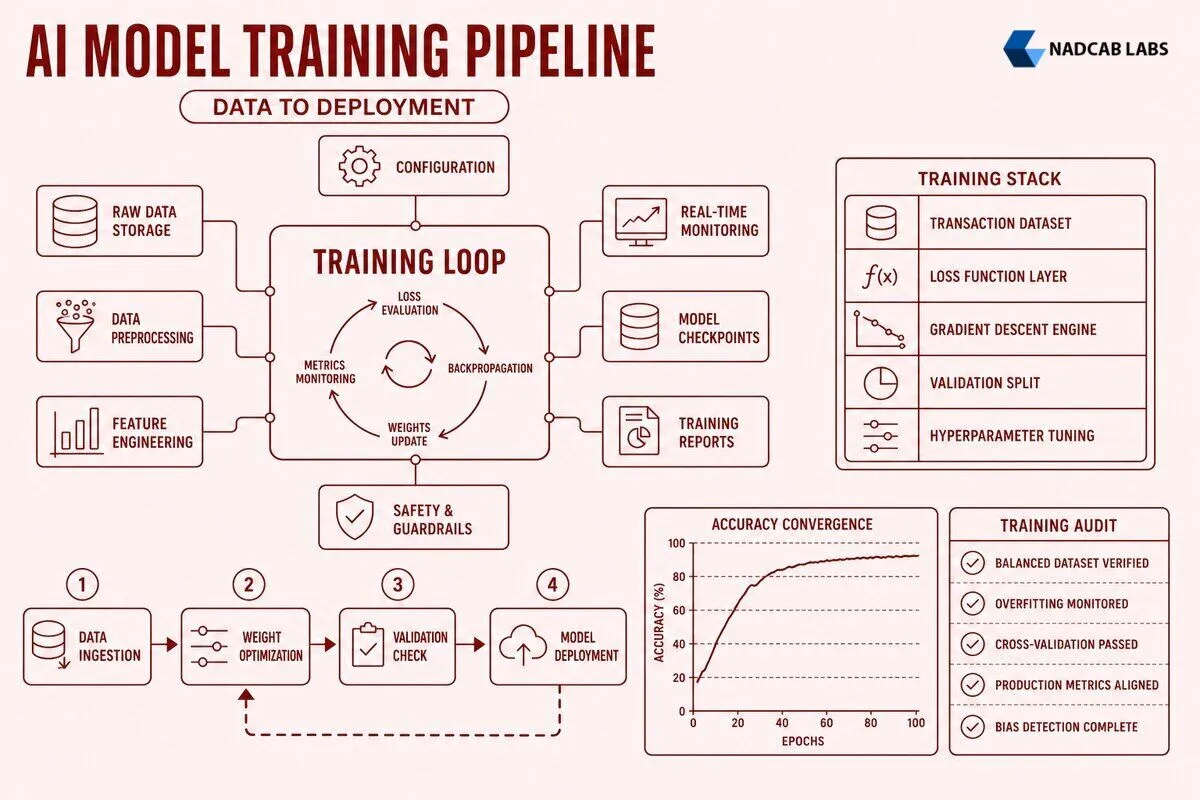
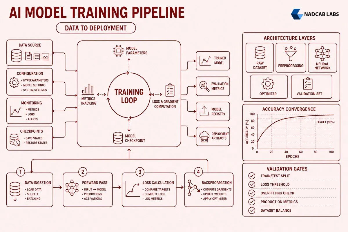
A model training pipeline consists of five sequential stages: data ingestion, feature engineering, training loop execution, validation and checkpointing, and final model export. Failures in any stage cascade downstream and degrade final model accuracy. ai model training.
Data ingestion pulls raw inputs from multiple sources: on chain event logs (Transfer events, Swap events, contract creation transactions), off chain API feeds (price oracles, social sentiment scores, centralized exchange order book snapshots), and labeled datasets (manually reviewed fraud cases, audited smart contracts with vulnerability tags). The ingestion layer must handle schema mismatches, missing values, and timestamp alignment across heterogeneous sources. ai model training.
For blockchain data, reorg handling is critical. A block you ingested may be orphaned, invalidating all derived features. You need logic to detect reorgs by comparing block hashes at depth N (typically 12 blocks on Ethereum) and purge any features derived from orphaned blocks. Rate limit backoff for RPC nodes prevents your pipeline from getting throttled mid ingestion. Deduplication matters when subscribing to multiple providers for redundancy; the same Transfer event may arrive twice with slightly different timestamps. ai model training.
Feature engineering converts raw data into numerical tensors the model can process. Categorical variables like token symbols or wallet addresses get encoded as integers via label encoding or one hot vectors. Continuous variables like transaction amounts get normalized to zero mean and unit variance to prevent large magnitude features from dominating gradient updates. ai model training.
The normalization parameters (mean and standard deviation) must be computed on the training set only, then applied to validation and test sets to avoid leakage. Graph features require aggregation: for a wallet, compute the mean, max, and standard deviation of incoming transfer amounts over the past 30 days, the count of unique counterparty addresses, and the eigenvector centrality score in the wallet interaction graph. ai model training.
Poor feature engineering is the number one cause of underperforming models. If your features do not capture the signal that distinguishes positive from negative examples, no amount of training will fix accuracy. A fraud detector trained on transaction amounts and timestamps alone will miss sophisticated attacks that exploit contract interaction patterns or multi hop token swaps. ai model training.
The training loop iterates over batches of examples, computing predictions, measuring error via a loss function, and updating model weights via backpropagation. A single training epoch processes the entire dataset once. Modern pipelines run 50 to 500 epochs depending on dataset size and model capacity.
Inside each iteration: the forward pass multiplies input features by weight matrices, applies activation functions (ReLU, sigmoid, softmax), and produces a prediction vector. The loss function compares predictions to ground truth labels, outputting a scalar error. For binary classification (fraud versus legitimate), cross entropy loss is standard. For regression (predicting gas price), mean squared error measures the average squared difference between predicted and actual values.
The backward pass computes gradients of the loss with respect to every weight using the chain rule, then an optimizer (SGD, Adam, AdamW) updates weights in the direction that reduces loss. Learning rate controls step size: too high causes divergence (loss explodes to infinity), too low causes slow convergence (the model takes 10x more epochs to reach the same accuracy).
State changes per epoch include weight tensors (the model parameters being optimized), gradient norms (the magnitude of weight updates, useful for diagnosing vanishing or exploding gradients), optimizer state (momentum buffers for Adam, moving averages of gradients and squared gradients), and learning rate schedules (cosine annealing, step decay, or warmup followed by exponential decay).
Checkpoint saving writes model state to disk every N epochs so you can resume training after a crash or roll back to an earlier checkpoint if validation loss starts increasing. Early stopping logic monitors validation loss: if it does not improve for K consecutive epochs, training halts to prevent overfitting. A typical K value is 10 to 20 epochs for small datasets, 5 to 10 for large datasets where each epoch is expensive.
| Pipeline Stage | Input | Output | Failure Mode | Validation Step |
|---|---|---|---|---|
| Data Ingestion | Event logs, API feeds, labels | Raw dataset (CSV, Parquet) | Schema drift, missing timestamps, reorgs invalidating blocks | Check row count, null percentage, verify block hash continuity |
| Feature Engineering | Raw dataset | Feature matrix (NumPy array) | High cardinality categoricals, skewed distributions, normalization leakage | Plot histograms, check for inf/NaN, verify train/val split integrity |
| Train/Val/Test Split | Feature matrix, labels | Three disjoint subsets (70/15/15) | Data leakage, class imbalance, temporal ordering violations | Verify no overlap, check class ratios, ensure chronological splits |
| Training Loop | Train set, initial weights | Trained weights, loss curve | Exploding gradients, NaN loss, learning rate too high | Monitor gradient norms, clip if >5.0, track loss every 10 batches |
| Validation & Checkpointing | Val set, trained weights | Val loss, saved checkpoint | Overfitting, checkpoint corruption, disk I/O errors | Compare train vs val loss, verify checkpoint loads, test restore |
| Model Export | Best checkpoint | Serialized model (ONNX, TorchScript) | Version mismatch, missing metadata, quantization errors | Run inference on test set, check latency, validate output shape |
You ingest raw data from your sources, engineer features that capture the signal you care about, split the data into train, validation, and test sets, run the training loop until convergence, validate and checkpoint periodically, then export the final model. Failures in early stages (bad features, leaky splits) cannot be fixed by tuning hyperparameters in the training loop. Always validate intermediate outputs before proceeding to the next stage.
Detecting Overfitting, Underfitting, and Data Drift
A lending protocol trains a default risk model on loan data from 2024. In the lab, training accuracy reaches 96% and validation accuracy hits 88%. Three months after deployment, the model’s precision drops to 62% as new borrower profiles emerge that differ from the training distribution.
The team did not monitor for drift. They only discovered the problem after manually reviewing a sample of flagged loans and noticing that most false positives came from wallets that had interacted with protocols launched after the training cutoff date.
Overfitting happens when a model learns to memorize training examples rather than generalize patterns. You see training loss continuing to decrease while validation loss plateaus or increases after a certain epoch. Numerically, you might see training accuracy at 95% but validation accuracy stuck at 68%. The model has high variance: it fits noise in the training set that does not exist in unseen data.
Root causes? Model capacity too high relative to dataset size (a 10 layer neural network trained on 500 examples will memorize every example). Insufficient regularization (no dropout, no weight decay) allows the model to assign arbitrarily large weights to spurious correlations. Training for too many epochs without early stopping gives the model time to overfit even if capacity is reasonable.
Fixes: Add L2 regularization by penalizing large weights (add a term to the loss function equal to the sum of squared weights multiplied by a small coefficient like 0.001). Apply dropout by randomly zeroing out neuron activations during training to prevent co adaptation (dropout rate of 0.3 to 0.5 is typical). Reduce model size by removing layers or narrowing layers (fewer neurons per layer). Use data augmentation to artificially expand the training set. For images: rotate, crop, flip. For blockchain data: add Gaussian noise to transaction amounts, permute transaction order within a block, or synthesize new examples by interpolating between existing feature vectors.
Underfitting occurs when the model lacks capacity to capture the underlying pattern. Both training and validation loss remain high. Training accuracy might be 65% and validation accuracy 62%, indicating the model is not learning much beyond random guessing.
Common causes: Model too simple (a linear classifier cannot learn a nonlinear decision boundary). Poor feature selection (you are missing the signal that separates classes; for example, trying to detect fraud using only transaction timestamps without amounts or counterparty information). Insufficient training (you stopped after 5 epochs when convergence requires 50). Noisy labels (ground truth annotations are inconsistent or wrong, so the model cannot learn a coherent pattern).
Remedies: Increase model capacity by adding layers or widening layers. Engineer better features. For fraud detection, add graph centrality metrics (PageRank, betweenness centrality) and transaction velocity features (number of transactions in the past hour, rolling average of transaction amounts). Train longer by monitoring loss curves to ensure they are still decreasing. Clean labels by reviewing a sample, correcting errors, or using semi supervised learning to take advantage of unlabeled data.
Data drift in production means the distribution of input features or the relationship between features and labels has shifted since training. Two types: covariate shift (feature distributions change but the decision boundary stays the same) and concept drift (the relationship between features and labels changes).
Example of covariate shift: you trained a gas price predictor on mainnet Ethereum data, then deployed on a Layer 2 rollup where transaction patterns differ (lower base fees, different congestion dynamics). The model’s features (recent block gas usage, pending transaction count) have different distributions on the new chain, but the relationship between those features and gas price is similar.
Example of concept drift: a fraud model trained in 2024 when phishing attacks used email links, but attackers in 2026 use social engineering via Discord DMs, so the features that indicated fraud in 2024 (transaction initiated from email click) no longer correlate with fraud (transaction initiated from Discord link).
Detection strategies: Monitor prediction confidence distributions. If your classifier’s mean predicted probability for the positive class drops from 0.7 to 0.4, the model is less certain, signaling possible drift. Track feature statistics: compute mean and standard deviation of each feature on a rolling 7 day window; alert if any feature’s mean shifts more than 2 standard deviations from training baseline. Measure performance metrics on recent data: compute F1 score, precision, recall on the past 1,000 predictions; trigger retrain if F1 drops more than 5% relative to validation set F1.
Automated retrain triggers: set a threshold (for example, retrain when validation F1 on recent data falls below 0.80) and schedule periodic retraining (weekly or monthly) even if metrics have not degraded, to keep the model fresh as new patterns emerge.
Comparison of diagnostic signals:
Production debugging workflow: when a model underperforms, first check recent prediction logs for anomalies (sudden spike in predictions of one class, confidence scores near 0.5 indicating uncertainty). Next, sample 100 recent examples the model got wrong and manually inspect features and labels to identify patterns. Are all errors concentrated in a specific wallet type or transaction size range?
Then compute feature distributions on recent data and compare to training set distributions using statistical tests like Kolmogorov Smirnov or chi squared. If drift is confirmed, retrain on a dataset that includes recent examples. If labels are unavailable for recent data, use active learning: have the model flag high uncertainty examples, manually label a small batch (say 200 examples), and fine tune the model on that batch.
Supervised vs. Unsupervised Training for Blockchain Use Cases
An NFT marketplace wants to cluster users by behavior to personalize homepage recommendations. They have transaction logs for 200,000 wallets but no labels indicating user intent (collector, flipper, artist). Supervised learning is not an option because labeling 200,000 wallets manually would cost months of analyst time.
Instead, they apply unsupervised clustering (K means or DBSCAN) on features like average hold time, transaction frequency, and collection diversity. The algorithm groups wallets into five clusters. Domain experts review a sample from each cluster and assign semantic labels: cluster 1 is long term collectors (high hold time, low frequency), cluster 2 is flippers (low hold time, high frequency), cluster 3 is artists (many mints, few purchases), and so on.
The team then builds a supervised classifier on 500 labeled examples (100 per cluster) and applies it to the remaining 199,500 wallets, effectively scaling their labels.
Supervised learning requires labeled training data: each example has input features and a known output label. The model learns a mapping from features to labels by minimizing prediction error on the training set. Use supervised learning when you have ground truth labels and a clear classification or regression task.
Blockchain examples: fraud detection (label: fraud or legitimate), transaction categorization (label: DeFi, NFT, token transfer, contract deployment), smart contract vulnerability scoring (label: critical, high, medium, low risk), gas price prediction (label: actual gas price in Gwei at a future timestamp).
Supervised methods include logistic regression, decision trees, random forests, gradient boosting machines, and neural networks. Accuracy depends on label quality and quantity: with 10,000 balanced labeled examples, a well tuned gradient boosting model can achieve 85% to 95% test accuracy on most blockchain classification tasks. With fewer than 1,000 examples, accuracy drops below 75% unless you use transfer learning (start from a model pre trained on a related task) or data augmentation.
Unsupervised learning finds structure in data without labels. The model groups similar examples (clustering) or reduces dimensionality (PCA, autoencoders) or detects outliers (isolation forest, one class SVM). Use unsupervised learning when labels are expensive, unavailable, or you want to discover novel patterns.
Blockchain examples: wallet clustering (group wallets by on chain behavior for targeted airdrops or Sybil detection), anomaly detection in DeFi protocols (flag unusual liquidity withdrawals or flash loan patterns that do not match historical norms), market regime identification (cluster time periods by volatility and correlation structure to switch trading strategies).
Unsupervised methods do not output accuracy metrics because there is no ground truth to compare against. Instead, evaluate using domain expert validation (do the clusters make sense?), silhouette score (how well separated are clusters?), or downstream task performance (if you use clusters as features in a supervised model, does accuracy improve?).
| Criterion | Supervised Learning | Unsupervised Learning |
|---|---|---|
| Label Requirement | Requires labeled data (10K+ samples for good accuracy) | No labels needed |
| Typical Accuracy | 85 to 95% on test set with quality labels | No accuracy metric; evaluated by cluster coherence or expert review |
| Common Algorithms | Logistic regression, XGBoost, neural networks | K means, DBSCAN, PCA, isolation forest |
| Blockchain Use Case | Fraud detection, smart contract risk scoring, transaction categorization | Wallet clustering, anomaly detection, market regime identification |
| Training Time | Hours to days depending on dataset size and model complexity | Minutes to hours; clustering scales to millions of examples |
| Interpretability | High for linear models, low for deep networks | Moderate; clusters can be profiled by feature means |
| Deployment Complexity | Moderate; need inference API and monitoring | Low; often run offline as batch jobs |
Hybrid approaches combine supervised and unsupervised methods. Semi supervised learning uses a small labeled set plus a large unlabeled set: train a supervised model on labeled data, use it to pseudo label high confidence unlabeled examples, then retrain on the expanded dataset.
Active learning iteratively selects the most informative unlabeled examples (high prediction uncertainty or near decision boundary), asks a human to label them, and retrains. Both techniques reduce labeling cost while improving accuracy.
For blockchain teams with limited annotation budget, start with unsupervised clustering to identify distinct wallet segments, then manually label a small sample from each cluster (say 100 examples per cluster), and train a supervised classifier on those labeled examples. The classifier can then predict cluster membership for all remaining wallets, effectively scaling your labels.
Decision tree: if you have 10,000+ labeled examples and a clear target variable (fraud yes/no, risk score 1 to 5), use supervised learning. If labels are unavailable or you want to explore data structure without a predefined task, use unsupervised learning. If you have a small labeled set (500 examples) and a large unlabeled set (500,000 examples), use semi supervised or active learning.
For real time production systems that need sub 100ms latency, supervised models (especially tree based ensembles or small neural networks) are easier to deploy than clustering pipelines. For offline analytics and exploratory analysis, unsupervised methods provide fast insights without the overhead of label collection.
Moving from Prototype to Production Ready Models
A wallet provider builds a fraud detection prototype that achieves 82% F1 score on a validation set. The team wants to deploy it to production but faces three blockers: the model was trained with default hyperparameters (learning rate 0.001, batch size 32) and no tuning, the inference latency is 450ms per prediction (too slow for real time transaction screening), and there is no monitoring or retrain pipeline.
After one week of tuning, they find that learning rate 0.0005 with batch size 64 and dropout 0.3 raises F1 to 91%. Quantizing the model from float32 to int8 and deploying on a 4 core CPU instance brings p99 latency down to 78ms. They set up a dashboard that tracks daily F1 on recent predictions and triggers a retrain if F1 drops below 0.85.
Hyperparameter tuning searches the space of training configurations to find the combination that maximizes validation performance. Key hyperparameters: learning rate (controls step size in gradient descent; typical range 0.0001 to 0.1), batch size (number of examples per gradient update; typical range 16 to 512), number of layers and neurons (model capacity), regularization strength (L2 penalty coefficient; typical range 0.0001 to 0.01), and dropout rate (fraction of neurons to zero out; typical range 0.1 to 0.5).
Tuning methods: grid search (try every combination in a predefined grid; exhaustive but slow), random search (sample random combinations; faster and often finds good configs), and Bayesian optimization (model the performance surface and sample points likely to improve; most sample efficient). A typical tuning run evaluates 50 to 200 configurations. Expect 20% to 50% accuracy gain over default hyperparameters. A fraud classifier might improve from 82% F1 to 91% F1 after tuning learning rate from 0.001 to 0.0005 and adding dropout 0.3.
Model serving architecture determines how predictions are delivered to applications. Two main patterns: REST API (synchronous request/response; client sends feature vector, server returns prediction in under 100ms) and batch inference (process a large dataset offline, write predictions to a database or file).
REST API is required for real time use cases like transaction screening or dynamic pricing. Batch inference suffices for offline analytics like daily wallet risk scoring. Latency budget: for REST API, aim for p99 latency under 100ms. This requires optimizing model size (quantize weights from float32 to int8, prune unnecessary neurons) and serving infrastructure (use a fast inference runtime like ONNX Runtime or TensorRT, deploy on GPU if model is large, or use CPU with multi threading if model is small).
Cost per inference: GPU inference costs roughly $0.0001 to $0.001 per prediction depending on model size and batch size; CPU inference costs $0.00001 to $0.0001 per prediction. For high volume applications (millions of predictions per day), CPU serving is more cost effective unless the model requires GPU for acceptable latency.
Integration with Model Training services offloads the heavy lifting of experiment tracking, distributed training, and continuous retraining. Experiment tracking logs every training run’s hyperparameters, metrics, and artifacts (model checkpoints, loss curves) so you can compare runs and reproduce results.
Distributed training splits a large dataset across multiple GPUs or nodes to reduce training time from days to hours. Continuous retraining pipelines automatically retrain the model when drift is detected or on a schedule (weekly, monthly), then deploy the new version if it outperforms the current production model.
By integrating with a managed service, a two person team can achieve high model quality and uptime without hiring a dedicated ML ops engineer. Time to production drops from 3 to 6 months (building everything in house) to 2 to 4 weeks using a service for training infrastructure and monitoring.
Production checklist before deploying a model:
Concrete next action for blockchain teams: if you have a prototype model, run hyperparameter tuning this week using a tool like Optuna or Ray Tune. If your model is already tuned, profile inference latency and optimize until p99 is under your budget. If you are building a new model from scratch, start by defining the task (classification, regression, clustering), collecting and labeling 1,000 examples, and training a baseline model with default hyperparameters to establish a performance floor.
Then iterate: add features, tune hyperparameters, and validate on recent data. For teams that need to ship fast, consider integrating Model Training services early in the project to avoid reinventing infrastructure.
Related blockchain ML use cases: What Is Blockchain in E Commerce? Benefits, Use Cases, and How It Works in 2026 discusses how trained models power fraud detection in payment systems. EHR interoperability blockchain cost covers data quality challenges similar to those in blockchain training datasets. modular blockchain interoperability explores cross chain data flows that require models to handle heterogeneous feature spaces. supply chain API integration costs examines API latency budgets relevant to model serving. private blockchain architecture design patterns includes sections on privacy preserving model training. Top NFT Marketplaces describes recommendation systems built on clustering and collaborative filtering. modular blockchain solutions often require models to adapt to new execution layers. Blockchain Identity Management systems use trained classifiers to detect identity fraud and Sybil attacks.
Summary
AI model training transforms raw blockchain data into predictive functions that power fraud detection, risk scoring, and on chain analytics. The training pipeline consists of data ingestion, feature engineering, iterative weight updates via backpropagation, validation, and checkpointing. Production failures stem from overfitting (memorizing noise), underfitting (insufficient capacity), or data drift (distribution shifts over time).
Supervised learning excels when you have labeled data and a clear target; unsupervised methods discover structure without labels. Moving from prototype to production requires hyperparameter tuning, low latency serving infrastructure, and continuous monitoring. Blockchain teams that integrate Model Training services reduce time to deployment and achieve higher accuracy than building everything in house.
Start by defining your task, collecting 1,000 labeled examples, training a baseline model, and iterating on features and hyperparameters until validation metrics meet your threshold.
Frequently Asked Questions
Q1.What is the difference between training data and validation data in AI model training?
Training data teaches the model patterns by adjusting weights through backpropagation across multiple epochs. Validation data evaluates performance on unseen examples during training to tune hyperparameters like learning rate or regularization strength. Validation loss diverging from training loss signals overfitting. Never use validation samples for gradient updates; they serve only as a checkpoint to measure generalization before final test set evaluation.
Q2.How do you prevent overfitting when training machine learning models on blockchain data?
Apply L2 regularization to penalize large weights, use dropout layers (0.3 to 0.5 rate) to randomly disable neurons, and implement early stopping when validation loss stops improving for five consecutive epochs. Augment transaction datasets by resampling minority classes or adding Gaussian noise to numeric features. Cross validate on different chain segments to ensure the model generalizes across block ranges and network conditions, not just memorizes historical patterns.
Q3.What loss functions work best for crypto fraud detection models?
Binary cross entropy suits binary fraud/legitimate classification, but class imbalance demands focal loss to down-weight easy negatives and focus on hard fraud cases. For multi-class scam taxonomy (phishing, rug pull, wash trading), use categorical cross entropy with class weights inversely proportional to sample frequency. Evaluate with precision-recall AUC, not accuracy, because legitimate transactions vastly outnumber fraud; a 99% accuracy model might miss every scam.
Q4.How much labeled data do you need to train an accurate AI model for smart contract analysis?
Minimum 5,000 labeled contracts for simple vulnerability binary classifiers; 50,000+ for multi-class bug taxonomy with acceptable recall. Transformer architectures parsing Solidity AST require 100,000+ examples to learn semantic patterns. Use semi-supervised learning: pre-train on millions of unlabeled contracts via masked language modeling, then fine-tune on your labeled set. Active learning helps; label high-uncertainty predictions first to maximize information gain per annotation hour.
Q5.What causes model drift in production and how do you detect it early?
Drift occurs when input distributions shift (new token standards, protocol upgrades, attacker tactics evolve) or when target relationships change (DeFi market regime shifts). Monitor prediction confidence distributions; sudden drops indicate unfamiliar inputs. Track feature statistics: if mean gas price or transaction value percentiles deviate beyond two standard deviations from training baselines, retrain. Compare live prediction error against holdout test error weekly; sustained increases above 15% signal drift requiring model updates.
Q6.When should blockchain teams use supervised vs unsupervised learning approaches?
Use supervised learning when you have labeled ground truth: fraud tags, verified contract bugs, known wallet clusters. It delivers higher accuracy for classification and regression tasks. Choose unsupervised methods (k-means, DBSCAN, autoencoders) for exploratory analysis without labels: discovering transaction patterns, clustering similar contracts, detecting anomalies in mempool behavior. Combine both: unsupervised clustering to identify candidate fraud rings, then supervised classifier to score each cluster member’s risk probability.
Explore Services
Related Services
Reviewed by

Aman Vaths
Founder of Nadcab Labs
Aman Vaths is the Founder & CTO of Nadcab Labs, a global digital engineering company delivering enterprise-grade solutions across AI, Web3, Blockchain, Big Data, Cloud, Cybersecurity, and Modern Application Development. With deep technical leadership and product innovation experience, Aman has positioned Nadcab Labs as one of the most advanced engineering companies driving the next era of intelligent, secure, and scalable software systems. Under his leadership, Nadcab Labs has built 2,000+ global projects across sectors including fintech, banking, healthcare, real estate, logistics, gaming, manufacturing, and next-generation DePIN networks. Aman’s strength lies in architecting high-performance systems, end-to-end platform engineering, and designing enterprise solutions that operate at global scale.