Ai Overview
At 3:47 AM, a cryptocurrency exchange’s risk dashboard froze mid flash crash. Traders watched their hedging signals stall for fifteen minutes. By the time the system caught up, the firm had bled through unhedged exposure worth six figures. Row formats force the query engine to read and discard 80% of the data.
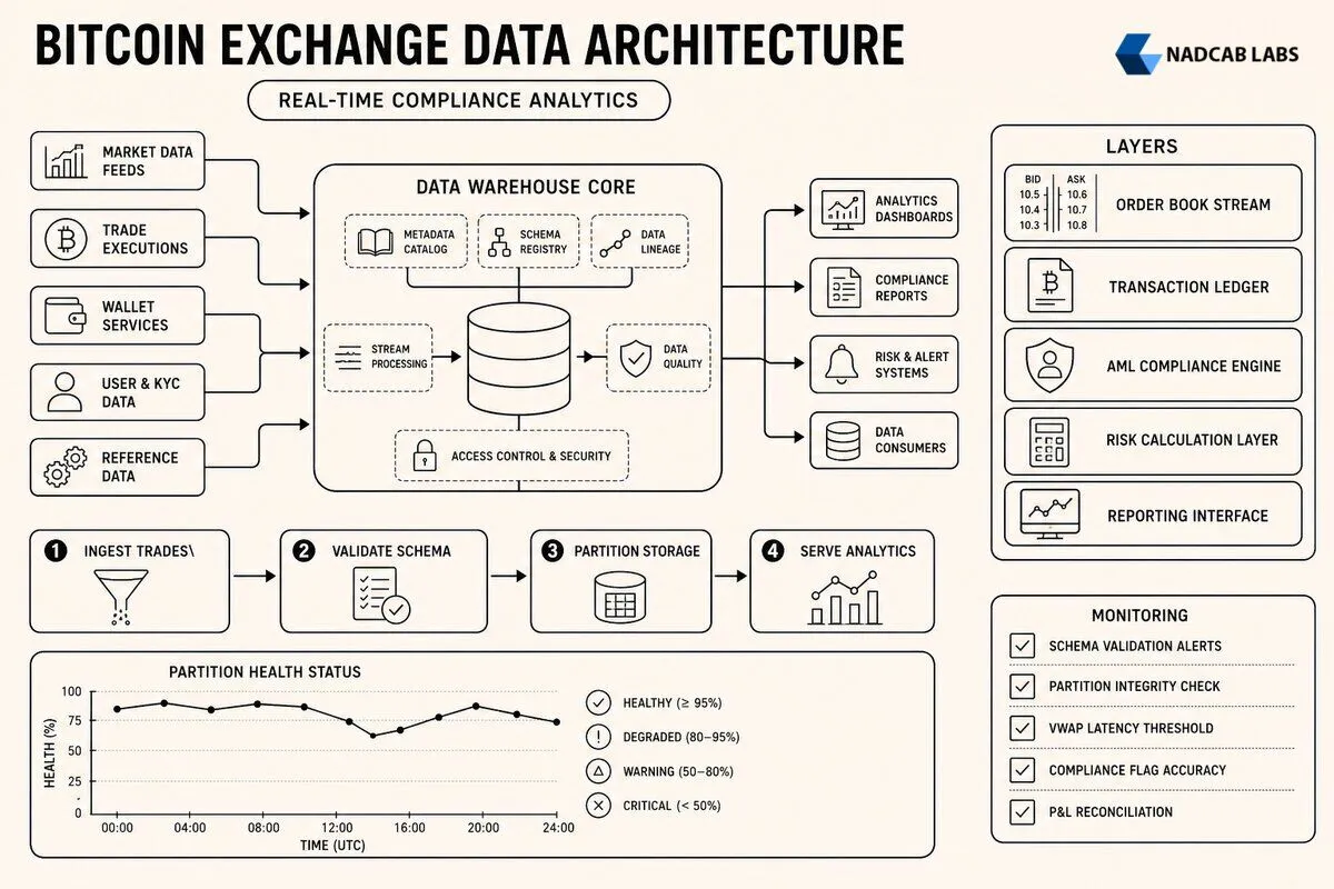
At 3:47 AM, a cryptocurrency exchange’s risk dashboard froze mid flash crash. Traders watched their hedging signals stall for fifteen minutes. By the time the system caught up, the firm had bled through unhedged exposure worth six figures. The culprit? A schema validation failure in their bitcoin exchange data warehouse had cascaded silently into every downstream analytics tool. The broken partition went undetected because no one had wired up alerts on partition health. This wasn’t a freak accident. It revealed what most exchanges discover the hard way: your warehouse isn’t passive storage. It’s the system that decides whether compliance sees accurate AML flags, whether quants get sub second VWAP calculations, and whether your CFO trusts the P&L enough to sign quarterly filings.
Key Takeaways
- Bitcoin exchange data warehouses must reconcile blockchain finality delays with sub second trading analytics. This forces hybrid ingest patterns: streaming order books paired with batch blockchain confirmations.
- Schema evolution becomes a production risk when adding new trading pairs or Lightning Network support. SCD Type 2 dimensions prevent historical query breakage during backfills.
- Columnar storage formats like Parquet reduce scan costs by 80% for time series aggregations. Partition strategy determines whether your dashboard refreshes in 200 milliseconds or times out.
- Data quality checks must run inline during ingestion. Sequence number gaps, cross system balance reconciliation, and null rate thresholds catch pipeline drift before traders see corrupt KPIs.
- Production observability requires lineage tracking from blockchain node through Kafka to warehouse. Automated alerts on SLA breaches need runbooks for on call engineers.
- Platforms like grovex btc demonstrate how enterprise grade warehouse architecture supports ML model training, regulatory reporting, and real time risk management in a single unified layer.
Why Bitcoin Exchange Data Warehouses Matter for Trading Analytics
When a compliance officer pulls an AML report at 9 AM and sees transaction counts that don’t match the blockchain explorer by 4,000 records, it’s not a rounding error. It signals a broken trust boundary between operational systems and analytical infrastructure. Bitcoin exchanges generate three distinct data streams that must converge in the warehouse: internal order state changes from the matching engine, market data feeds from external venues for arbitrage signals, and on chain transaction confirmations from full nodes. Each stream operates on different clocks. The matching engine emits microsecond timestamps. Blockchain confirmations arrive in ten minute intervals with probabilistic finality. Market data feeds from other exchanges may lag by 50 to 200 milliseconds depending on API tier.
Stale dashboards cost exchanges in concrete ways. A risk manager relying on 15 minute old position data cannot execute dynamic hedging strategies during volatility spikes. A quant team training ML models on yesterday’s tick data will deploy strategies that assume liquidity patterns already obsolete by morning. Regulatory auditors demand point in time snapshots of user balances, withdrawal queues, and KYC status as of specific block heights. This requires the warehouse to store every state transition with blockchain height metadata. Missing this dimension means you cannot prove compliance during an investigation. bitcoin exchange.
Platforms like GroveX structure their warehouses to support three concurrent workloads: real time dashboards for traders viewing sub second P&L updates, batch ML pipelines that retrain models overnight on 90 days of tick data, and ad hoc analyst queries that scan six months of order history to identify wash trading patterns. Real time queries need hot data in memory with minimal join complexity. ML pipelines require full table scans across compressed columnar files. Analyst queries need flexible schema on read semantics to explore dimensions not anticipated during initial design. A well architected bitcoin exchange data warehouse serves all three without forcing teams into separate siloed systems.
The unique challenge of BTC data is cardinality explosion. A single trading pair like BTC/USDT generates 50,000 order book updates per second during high volatility. Each update contains bid and ask ladders with 20 to 50 price levels. Storing raw snapshots at this granularity produces billions of rows per day for one pair. Aggregating too aggressively loses the tick level precision needed for market microstructure research. You face a choice: store every snapshot and accept massive monthly growth, or sample at one second intervals and risk missing the exact sequence that triggered a liquidation cascade. Your answer determines whether your post mortem after a flash crash can reconstruct causality or just shows a gap in the data. bitcoin exchange.
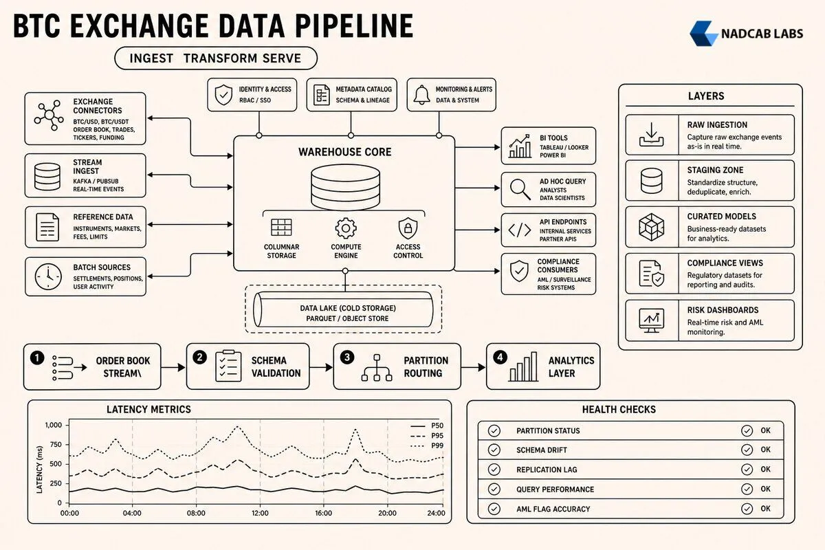
Ingest Layer: Capturing Bitcoin Trade & Blockchain Data at Scale
The ingest layer is where most data quality problems originate, because it sits at the boundary between systems you control and external dependencies you don’t. A production grade bitcoin exchange data warehouse ingests from four primary sources: the internal matching engine via database change data capture, WebSocket feeds from the exchange’s own public API for order book snapshots, blockchain full nodes polled every block for deposit and withdrawal confirmations, and external market data providers for cross venue arbitrage signals. Each source has different failure modes and requires distinct SLA contracts.
Stream ingestion through Kafka topics works well for high frequency data like order book updates and trade executions. The matching engine publishes every state change to a Kafka topic partitioned by trading pair, ensuring order within each partition while allowing parallel consumption. A typical setup uses three topics: orders.created for new limit and market orders, orders.matched for executed trades with maker and taker sides, and orders.cancelled for user cancellations and system timeouts. Every message includes a monotonically increasing sequence number per partition. Consumers track the last processed sequence number in a checkpoint table. On restart, they resume from the checkpoint. When a consumer detects a gap in sequence numbers, it triggers an alert and enters backfill mode, requesting missing messages from Kafka’s retention window. bitcoin exchange.
Batch ingestion handles blockchain data where latency tolerance is higher but correctness is non negotiable. A full Bitcoin node exposes RPC endpoints to query blocks, transactions, and mempool state. The warehouse polls getblockcount every 30 seconds. When a new block appears, it fetches the full block with getblock and extracts all transactions. The system checks each transaction against the exchange’s known deposit addresses. Confirmed deposits update user balances in the operational database and simultaneously land in a staging table in the warehouse. The staging table includes the block hash, block height, and confirmation count. Only after six confirmations does the deposit move from staging to the main fact table, preventing reorg induced double counting. bitcoin exchange.
Schema on read versus schema on write is a decision you make at the ingest boundary. Schema on write enforces structure during ingestion: every incoming message must match a predefined Avro or Protobuf schema, and any mismatch triggers a dead letter queue. This approach catches data corruption early but requires schema evolution coordination across producer and consumer teams. Schema on read stores raw JSON or binary blobs in the warehouse and applies structure during query time. This flexibility allows analysts to explore new fields without waiting for schema updates, but it pushes validation downstream, risking that corrupt data propagates into dashboards before anyone notices. bitcoin exchange.
For bitcoin exchange data warehouse architectures, a hybrid approach works best. Use schema on write for high volume, well understood streams like trades and orders, where the cost of schema drift is high. Use schema on read for exploratory data like mempool events or Lightning Network channel state, where the schema is still evolving. This split allows the core analytics pipeline to maintain strict SLAs while giving researchers access to experimental data sources.
SLA targets for the ingest layer must account for external dependencies. Internal matching engine data should land in the warehouse within two seconds of the event timestamp, measured as the delta between the event’s created_at field and the warehouse row’s ingested_at timestamp. Blockchain data has a different SLA: deposits must appear in the staging table within 60 seconds of block propagation, and move to the confirmed state within 90 minutes (six blocks at ten minutes each, plus processing overhead). External market data feeds are best effort: if an API rate limit is hit, the ingestion job backs off exponentially and logs the gap for manual review. bitcoin exchange.
Failure mode detection requires inline validation at every stage. After consuming a batch of Kafka messages, the ingestion job compares the count of messages processed against the difference in sequence numbers. If the count is lower, messages were dropped in flight, possibly due to a network partition or a bug in the serialization layer. After polling a blockchain node, the job verifies that the new block’s previousblockhash matches the hash of the last ingested block. A mismatch indicates either a reorg or that the node is out of sync. In both cases, the job halts and pages the on call engineer rather than silently writing corrupt data. bitcoin exchange.
| Data Source | Ingestion Method | SLA Target | Failure Mode | Detection Method |
|---|---|---|---|---|
| Matching Engine Orders | Kafka CDC stream | 2 seconds end to end | Sequence number gap | Compare message count vs sequence delta |
| Order Book Snapshots | WebSocket feed to Kafka | 500 milliseconds | WebSocket disconnect | Heartbeat timeout, reconnect with backfill |
| Blockchain Deposits | RPC poll every 30 seconds | 60 seconds to staging | Node out of sync or reorg | Verify previousblockhash linkage |
| External Market Data | REST API batch fetch | Best effort, 5 minute lag acceptable | API rate limit or downtime | Exponential backoff, log gap for review |
Transform & Model: Star Schema Design for Bitcoin Trading Data
Raw data lands in staging tables. The transform layer reshapes it into a queryable star schema optimized for analytical workloads. The central fact table stores trades: each row represents one executed order match, with foreign keys to dimension tables for users, trading pairs, and timestamps. A second fact table captures order lifecycle events: creation, partial fills, cancellations, and expirations. A third fact table tracks deposits and withdrawals, linking blockchain transaction IDs to user accounts. Every fact table is append only and immutable after the initial insert, simplifying auditing and enabling time travel queries. bitcoin exchange.
Dimension tables provide descriptive context. The user dimension includes account ID, KYC tier, registration timestamp, and current jurisdiction. The trading pair dimension lists all supported pairs with base and quote asset metadata, tick size, and minimum order quantity. The wallet dimension maps blockchain addresses to user accounts, tracking ownership changes over time. The timestamp dimension breaks down each second into hour, day, week, month, and quarter for efficient date range filtering.
Handling schema evolution without breaking existing queries requires intentional versioning. When the exchange adds support for a new trading pair, the trading pair dimension gains a new row, but the fact table schema doesn’t change because it references pairs by ID. When the exchange starts supporting Lightning Network deposits, the deposit fact table needs a new nullable column for the Lightning invoice hash. Existing rows have NULL in this column. Queries that don’t care about Lightning can ignore the column. Queries that filter on Lightning invoices add a WHERE clause checking for non NULL values. This additive approach avoids the need to rewrite historical data.
Adding a new asset class like options or perpetual futures is more complex. Options have strike prices and expiration dates that don’t apply to spot trades. Creating a single unified fact table that handles both spot and derivatives leads to a sparse schema with many NULL columns. A better pattern is to create separate fact tables: fact_spot_trades and fact_options_trades, each with a schema tailored to its domain. Both tables share common dimensions like users and timestamps, but have different trading pair dimensions. This separation keeps queries fast and schemas readable.
Slowly Changing Dimensions handle attributes that change over time but require historical accuracy. User KYC status is a classic example. A user starts at tier 1, completes identity verification to reach tier 2, then later gets flagged for suspicious activity and downgraded to tier 0. Regulatory queries need to know the user’s tier at the exact moment of each trade. SCD Type 2 solves this by storing every version of the user record with valid_from and valid_to timestamps. The user dimension has multiple rows per user, each representing one state. Queries join the fact table to the dimension on user ID and filter where the trade timestamp falls between valid_from and valid_to. This pattern ensures that a historical query asking for all tier 2 trades in March returns the correct result even if those users have since changed tiers.
Backfills are inevitable when you discover a data quality issue or need to reprocess historical data with new transformation logic. The key is to make backfills idempotent and auditable. Every fact table row includes a batch_id field that records which ETL run inserted it. When reprocessing a date range, the backfill job deletes all rows with the old batch_id for that range and inserts new rows with a new batch_id. The batch metadata table logs the start time, end time, row count, and any validation errors for each batch. If the backfill fails midway, you can identify which date partitions are incomplete and rerun just those partitions without affecting the rest of the data.
For teams evaluating Data Warehouse Development, the transform layer is where business logic and data engineering intersect. A poorly designed schema forces analysts to write 15 line SQL queries with five joins just to calculate daily trading volume. A well designed schema lets them write SELECT SUM(quantity) FROM fact_trades WHERE trade_date = '2026 03 15' and get the answer in 200 milliseconds. The difference isn’t just convenience. It determines whether your data team can iterate fast enough to support product launches and regulatory deadlines.
Star Schema Transform Process Flow
Raw JSON/Avro messages land in staging tables partitioned by ingestion hour, preserving source format for replay.
Inline checks verify required fields, data types, and referential integrity; failed rows route to error queue with validation reason.
Enrich facts with dimension keys; new dimension members trigger SCD Type 2 inserts with valid_from timestamp.
Append validated, enriched rows to partitioned fact tables; record batch_id and processing timestamp for lineage.
Incrementally update aggregates for dashboards; compare row counts against source to detect drift.
Storage & Query Optimization: Columnar Formats and Partition Strategies
Storage format directly impacts query latency and infrastructure cost. Row oriented formats like CSV or JSON store each record as a contiguous block, which works well for transactional workloads that read entire rows. Analytical queries, however, typically scan millions of rows but only access a few columns. A query calculating daily average trade size reads the quantity and trade_date columns but ignores user ID, order ID, and price. Row formats force the query engine to read and discard 80% of the data.
Columnar formats like Parquet and ORC store each column separately, allowing the query engine to read only the columns it needs. Parquet uses dictionary encoding and run length encoding to compress repetitive values. A column storing trading pair IDs for BTC/USDT trades might have 50 million rows but only one distinct value, compressing to a few kilobytes. Parquet also supports predicate pushdown: if the query filters on trade_date = '2026 03 15', the storage layer reads only the row groups where the min/max statistics for trade_date overlap that value, skipping entire files without touching disk.
In practice, Parquet reduces scan costs by 70 to 85% compared to JSON for typical bitcoin exchange data warehouse queries. A query summing trade volume across all pairs for one day scans 12 GB of Parquet files versus 94 GB of JSON, completing in 3.2 seconds instead of 28 seconds on the same cluster. ORC offers similar compression but is optimized for Hive and Presto, while Parquet has broader ecosystem support including Spark, Snowflake, and BigQuery.
Partitioning strategy determines which files the query engine opens. Partitioning by trade_date is standard: each day’s data lives in a separate directory. A query filtering on one date reads only that partition. But partitioning by date alone is insufficient for high cardinality queries. A query analyzing BTC/USDT trades for one day still scans all trading pairs if the data isn’t further partitioned. Multi level partitioning by trade_date and trading_pair_id creates a directory tree where each leaf contains trades for one pair on one day. This reduces scan size by another 95% for pair specific queries.
Over partitioning, however, creates its own problems. If you partition by hour instead of day, a query spanning one week must open 168 partition directories. Each directory open incurs metadata overhead. Cloud storage systems like S3 charge per API call, so listing 168 directories costs more than listing seven. The optimal partition size balances scan reduction against metadata overhead. For bitcoin exchange data, daily partitions work well for fact tables with uniform write rates. Hourly partitions make sense only for extremely high volume pairs where daily files exceed 10 GB compressed.
Materialized views precompute expensive aggregations so dashboards don’t recalculate them on every page load. A view that sums hourly trade volume by pair can be refreshed incrementally: when new data arrives for hour H, only the rows for hour H are recalculated and merged into the view. The view stores the last refreshed timestamp. Queries against the view include a staleness check: if the view is more than five minutes old, the dashboard shows a warning. This prevents users from making decisions on stale data while allowing the view to refresh asynchronously in the background.
Incremental refresh logic must handle late arriving data. A trade executed at 14:58 UTC might not land in the warehouse until 15:03 due to network latency. If the materialized view for the 14:00 hour was already refreshed at 15:01, it missed that trade. The refresh job needs a lookback window: when refreshing hour 15, it also re scans hour 14 to catch any late arrivals. The lookback window should be at least twice the P99 ingestion latency. If 99% of trades land within 90 seconds, use a three minute lookback.
Query optimization for bitcoin trading analytics often involves denormalization trade offs. Joining the trade fact table to the user dimension to filter by KYC tier is expensive if done on every query. Pre joining the most common dimensions into a wide fact table speeds up queries but increases storage cost and complicates schema evolution. A middle ground is to create multiple fact tables optimized for different query patterns: a narrow fact table with just trade essentials for ML pipelines that scan billions of rows, and a wide fact table with pre joined dimensions for dashboard queries that scan thousands of rows but need rich filtering.
Query Latency by Storage Format and Partition Strategy
Benchmark: aggregate daily trade volume across all pairs, single date filter, 94 GB dataset, 8 node Spark cluster.
Governance & Observability: Ensuring Data Quality in Production
Data lineage tracking answers the question: where did this number come from? When a CFO sees a discrepancy between the exchange’s internal ledger and the data warehouse P&L report, the investigation starts with lineage. The warehouse must trace every fact table row back to its source: which Kafka message, which blockchain transaction, which API response. Lineage metadata includes the ingestion timestamp, the ETL job version, and the source system commit hash. If the discrepancy originated from a bug in the transform logic, you can identify all affected rows by filtering on the job version and trigger a targeted backfill.
Metadata catalogs like Apache Atlas or Amundsen store lineage graphs as directed acyclic graphs where nodes represent datasets and edges represent transformations. A query against the catalog shows that the daily_pnl dashboard reads from the user_pnl_summary materialized view, which aggregates the fact_trades table, which is populated by the kafka_trades_consumer job, which reads from the trades.matched Kafka topic, which is published by the matching engine. Every edge stores the transformation logic as a SQL or Spark query. This transparency lets analysts understand data freshness and trust boundaries without asking the engineering team.
Automated quality checks run inline during ingestion and transformation. Row count reconciliation compares the number of rows inserted into the fact table against the number of messages consumed from Kafka. A mismatch triggers an alert. Duplicate detection checks for rows with identical primary keys; duplicates indicate a bug in the deduplication logic or a Kafka producer retry that wasn’t idempotent. Null rate thresholds flag columns that should never be NULL: if more than 0.1% of trades have a NULL price, the pipeline halts and pages the on call engineer.
Cross system balance verification is critical for financial correctness. The warehouse sums all deposits, withdrawals, and trades for each user and compares the result against the operational database’s balance table. Any discrepancy larger than one satoshi indicates either a missing transaction in the warehouse or a bug in the operational system. This check runs hourly and logs discrepancies to a reconciliation queue. Small discrepancies under 1000 satoshis are often due to rounding differences in fee calculations and are reviewed manually. Large discrepancies trigger an immediate investigation.
Pipeline drift detection monitors for subtle degradation over time. Late arriving data is normal, but if the P99 ingestion latency increases from 90 seconds to 300 seconds over a week, it signals a problem: maybe the Kafka cluster is under provisioned, or the blockchain node is falling behind due to disk I/O saturation. Schema mismatches occur when a producer changes a field type without coordinating with consumers. If the matching engine starts sending quantity as a string instead of a decimal, the warehouse’s schema validation catches it and routes those messages to a dead letter queue. The alert includes the message payload and the validation error, giving the on call engineer enough context to file a bug report with the matching engine team.
SLA breach alerting ties each data pipeline stage to a measurable target and escalates when targets are missed. The ingest layer has a two second SLA. If the delta between event timestamp and ingestion timestamp exceeds two seconds for more than 5% of messages over a five minute window, an alert fires. The transform layer has a ten minute SLA: fact table rows must appear within ten minutes of the source event. The dashboard refresh layer has a 30 second SLA: materialized views must reflect data up to 30 seconds old. Every alert includes a runbook link that walks the on call engineer through diagnosis: check Kafka consumer lag, verify the blockchain node is synced, inspect the ETL job logs for errors, query the metadata catalog to identify downstream dependencies.
Runbooks are essential for on call effectiveness. A generic alert saying “warehouse ingestion slow” is useless at 3 AM. A specific alert saying “BTC/USDT order book ingestion latency P99 = 4.2 seconds, exceeds 2 second SLA, runbook: https://wiki.example.com/warehouse/btc orderbook latency” gives the engineer a starting point. The runbook lists common causes: WebSocket feed disconnected, Kafka partition rebalancing, downstream Snowflake cluster paused. It includes SQL queries to check the state of each component and commands to restart services if needed. Good runbooks turn a two hour debugging session into a 15 minute fix.
For exchanges building on platforms like grovex btc, observability is not optional. A production grade bitcoin exchange data warehouse must expose metrics at every layer: Kafka consumer lag per partition, blockchain node sync status, ETL job duration and row counts, query latency percentiles, and materialized view staleness. These metrics feed into dashboards that the data engineering team monitors during business hours and into alerting systems that wake up the on call engineer when SLAs are breached. Without this instrumentation, you’re flying blind, and the first sign of a problem is a trader complaining that the dashboard is wrong.
| Quality Check | Frequency | Threshold | Action on Breach |
|---|---|---|---|
| Row count reconciliation | Per batch (every 5 min) | Kafka messages = warehouse rows ± 0 | Halt pipeline, page on call, log discrepancy |
| Duplicate detection | Per batch | Duplicate primary keys = 0 | Halt pipeline, inspect deduplication logic |
| NULL rate threshold | Per batch | NULL in required columns < 0.1% | Alert, route bad rows to error queue |
| Cross system balance verification | Hourly | Warehouse balance = ledger balance ± 1 satoshi | Log to reconciliation queue, investigate if > 1000 sats |
| Ingestion latency P99 | Continuous (5 min window) | P99 < 2 seconds | Alert if > 5% of messages exceed threshold |
| Schema mismatch detection | Per message | 100% schema compliance | Route to dead letter queue, alert with payload sample |
| Materialized view staleness | Per query | Last refresh < 5 minutes ago | Display staleness warning on dashboard |
Before committing to a bitcoin exchange data warehouse architecture, evaluate your team’s ability to operate it. A warehouse isn’t a set and forget system. It requires continuous tuning, schema evolution, backfill management, and incident response. If your team lacks experience with distributed systems, start with a managed service like Snowflake or BigQuery that abstracts infrastructure complexity. If you need full control over storage format and query engine, consider a self hosted stack with Spark and Parquet on S3, but budget for the operational overhead. The decision criteria should weigh query performance requirements against operational maturity. A startup with two data engineers should not build a custom Presto cluster. A large exchange processing billions of trades per day may need that level of control to hit sub second dashboard SLAs.
The minimum viable warehouse for a new exchange includes daily batch ingestion from the operational database, a star schema with trade and user dimensions, Parquet storage partitioned by date, and basic quality checks on row counts and NULL rates. This setup supports regulatory reporting and basic analytics without the complexity of real time streaming. As trading volume grows, you add streaming ingestion, materialized views, and cross system reconciliation. The key is to build incrementally, validating each layer before adding the next, rather than attempting a big bang migration that introduces too many failure modes at once.
Exit criteria for a successful warehouse deployment include measurable SLAs met consistently over 30 days, zero data discrepancies between warehouse and operational systems during an audit, and analyst self service queries completing in under ten seconds for 95% of use cases. If you cannot meet these criteria, the warehouse isn’t production ready. Debugging should happen in a staging environment with synthetic data, not in production where bad data can trigger regulatory penalties or trading losses.
Related architectural patterns include Web3 Exchange Architecture for decentralized trading infrastructure, P2P exchange escrow smart contract architecture for trustless settlement, and Zero Knowledge Proof Real Estate Tokenization for privacy preserving analytics. Teams building Crypto Derivatives Exchange Development face similar warehouse challenges but with additional complexity from options Greeks and margin calculations. Integration with Data Science and ML Model Development Services requires feature stores that bridge the warehouse and model training pipelines, ensuring that models train on the same data analysts query. Security considerations overlap with crm data security frameworks, particularly around PII handling and access control. Even emerging use cases like bitcoin wallets ar vr integration depend on warehouse infrastructure to track user interactions and optimize UX.
Production bitcoin exchange data warehouses succeed when they balance three competing priorities: query performance for real time dashboards, cost efficiency for long term storage, and operational simplicity for small teams. Overengineering leads to systems that are too complex to debug. Underengineering leads to systems that cannot scale past the first million users. The right architecture depends on your specific constraints: trading volume, team size, regulatory requirements, and budget. Start with the simplest design that meets your current needs, instrument it thoroughly, and evolve it based on measured bottlenecks rather than hypothetical future requirements. bitcoin exchange, bitcoin exchange, bitcoin exchange.
Frequently Asked Questions
Q1.What is a Bitcoin exchange data warehouse and how does it differ from traditional OLTP databases?
A bitcoin exchange data warehouse is a read-optimized analytical store aggregating trade executions, order book snapshots, blockchain confirmations, and user activity for reporting and machine learning. Unlike OLTP databases that prioritize row-level writes and transactional consistency, warehouses use columnar storage (Parquet, ORC) and batch/micro-batch ingestion to scan billions of rows efficiently. OLTP handles live order matching; the warehouse reconstructs historical price candles, slippage metrics, and liquidity depth without impacting trading latency.
Q2.How do platforms like GroveX ingest real-time BTC trade data into a warehouse without losing tick-level precision?
GroveX streams trade events from the matching engine into Kafka topics partitioned by trading pair, preserving nanosecond timestamps and sequence numbers. A Flink or Spark Streaming job consumes each message, appends it to a staging Delta Lake table with ACID guarantees, then merges into the main fact table every 10 seconds. Exactly-once semantics via Kafka offsets and idempotent writes prevent duplicate ticks. Late-arriving trades trigger backfill jobs that rewrite affected partitions, maintaining tick-level precision for regulatory audit trails.
Q3.What schema design patterns work best for modeling Bitcoin transactions, order books, and blockchain confirmations?
Use a star schema: a central trades fact table (trade_id, timestamp, pair, price, quantity, taker_side, fee) joined to dimension tables for users, pairs, and fee tiers. Store order book snapshots in a separate time-series table partitioned by pair and minute, recording bid/ask arrays as JSON or nested structs. Blockchain confirmations live in a confirmations fact keyed by txid and block_height, linked to deposit/withdrawal events. Partition all tables by date and pair to prune scans; cluster by timestamp within partitions for range queries.
Q4.How can exchanges detect and recover from data pipeline failures that cause stale analytics dashboards?
Instrument each pipeline stage with heartbeat metrics: last processed Kafka offset, row counts per partition, and max event timestamp. Alerting triggers when the lag between wall-clock time and max event timestamp exceeds five minutes or row counts drop below historical percentiles. Recovery involves replaying Kafka from the last committed offset, recomputing affected partitions via idempotent SQL merges, and validating row checksums against the source OLTP replica. Automated backfill scripts compare warehouse aggregates to live database snapshots, flagging discrepancies for manual reconciliation.
Q5.What are the key SLA metrics for a production-grade crypto exchange data warehouse?
End to end latency under 60 seconds from trade execution to dashboard refresh, ensuring traders see near-live PnL. Query P95 latency below two seconds for standard reports (daily volume, top pairs). Data completeness above 99.99 percent, verified by reconciling warehouse trade counts against the matching engine’s append-only log. Schema migration downtime under five minutes per quarter. Disaster recovery RTO of four hours, with incremental snapshots replicated across three availability zones and point-in-time restore capability for the past 90 days.
Q6.How do you handle schema evolution when adding new trading pairs or blockchain networks to an existing warehouse?
Add columns with default null values using ALTER TABLE in systems like Delta Lake or Iceberg, which track schema versions per file. New pairs insert rows into the existing trades table; partition pruning isolates queries to relevant pairs. For blockchain networks, create a network_id dimension and foreign key in the confirmations table. Deploy schema changes via blue/green pipelines: write to both old and new schemas during a transition window, validate row parity, then cut over readers. Store schema metadata in a Git-versioned registry so downstream BI tools auto-refresh column definitions.
Explore Services
Related Services
Reviewed by

Aman Vaths
Founder of Nadcab Labs
Aman Vaths is the Founder & CTO of Nadcab Labs, a global digital engineering company delivering enterprise-grade solutions across AI, Web3, Blockchain, Big Data, Cloud, Cybersecurity, and Modern Application Development. With deep technical leadership and product innovation experience, Aman has positioned Nadcab Labs as one of the most advanced engineering companies driving the next era of intelligent, secure, and scalable software systems. Under his leadership, Nadcab Labs has built 2,000+ global projects across sectors including fintech, banking, healthcare, real estate, logistics, gaming, manufacturing, and next-generation DePIN networks. Aman’s strength lies in architecting high-performance systems, end-to-end platform engineering, and designing enterprise solutions that operate at global scale.