Ai Overview
Single-machine training is obsolete for frontier models: GPT-3 requires 355 GPU-years to train; no single machine can hold 175B parameters. NVIDIA GPUs have approximately 1% annual failure rate—with 1000 GPUs, expect failures every 3-4 days. At 8 GPUs (single node), achieving 95% efficiency is standard. Beyond 1000 GPUs, maintaining 70% efficiency requires heroic engineering.
Key Takeaways – Distributed Training Systems
- Single-machine training is obsolete for frontier models: GPT-3 requires 355 GPU-years to train; no single machine can hold 175B parameters. Distributed systems are mandatory, not optional.
- Three parallelism strategies address different bottlenecks: Data parallelism scales compute, model parallelism handles memory constraints, pipeline parallelism reduces idle time—modern systems combine all three.
- Communication often limits scaling more than computation: Beyond 100 GPUs, network bandwidth and gradient synchronization overhead dominate training time unless optimized aggressively.
- Synchronous vs asynchronous training involves fundamental trade-offs: Synchronous ensures consistency but requires perfect coordination; asynchronous tolerates stragglers but risks gradient staleness.
- Fault tolerance is critical at scale: With 1000+ GPUs running for weeks, failures are inevitable. Checkpointing and elastic training prevent catastrophic restart costs.
- Linear scaling is aspirational, not automatic: Doubling GPUs rarely doubles throughput due to communication overhead, synchronization costs, and diminishing batch size returns.
Introduction: Why Single-Machine Training No Longer Works
In 2018, training GPT-2 (1.5B parameters) on a high-end workstation was challenging but feasible. By 2020, GPT-3 (175B parameters) required cluster-scale infrastructure. In 2024, frontier models exceed a trillion parameters, consuming tens of thousands of GPUs running for months. The era of single-machine AI model training ended not gradually, but abruptly with the rise of large-scale architectures.
Three constraints drove this transition. First, model memory requirements: a 175B parameter model in FP32 consumes 700GB just for weights, exceeding any single GPU’s VRAM by 10x. Second, compute time: training on trillion-token datasets requires 10²⁴ floating-point operations—years on single GPUs. Third, dataset scale: modern training corpora exceed petabytes, demanding parallel data loading that saturates single-machine I/O.
Distributed training systems emerged not as optimization but necessity. Understanding these systems requires examining how computation, memory, and communication split across machines while maintaining training correctness and efficiency.
What “Distributed Training” Really Means in Practice
Distributed training encompasses multiple architectural patterns, each addressing different bottlenecks:
- Multi-GPU (single node): 2-8 GPUs connected via NVLink/PCIe, sharing system memory and fast interconnect
- Multi-node (cluster): Dozens to thousands of servers networked via InfiniBand or Ethernet, coordinating across data centers
- Multi-data-center: Geographically distributed training with high-latency WAN links (rare due to communication costs)
At the system level, distributed training partitions three resources: computation (which GPU processes which data/layers), memory (where parameters and gradients reside), and communication (how updates synchronize). Different parallelism strategies make different partitioning choices.
Core Building Blocks of Distributed Training Systems
Every distributed training system comprises five foundational components:
Distributed Training System Components
Workers execute training iterations. Parameter storage maintains model state (centralized in parameter servers or distributed across workers). Gradient exchange propagates updates (via All-Reduce, parameter servers, or hybrid approaches). Synchronization ensures consistency (synchronous for determinism, asynchronous for speed). Orchestration handles scheduling, fault recovery, and resource allocation.
Data Parallelism: Splitting the Dataset Across Machines
Data parallelism is the simplest and most common distributed training strategy. Each worker maintains a complete copy of the model and processes different data shards. After computing gradients locally, workers synchronize updates and apply averaged gradients to all model copies.
The process works as follows: partition dataset into N equal shards (one per worker), each worker performs forward pass on its shard computing loss, backward pass computes gradients, all workers exchange and average gradients via All-Reduce or parameter server, each worker updates its local model copy with averaged gradients. This ensures all workers maintain identical parameters despite processing different data.
Data parallelism scales effective batch size linearly with worker count. Using 8 GPUs with local batch size 32 creates effective batch size 256. This improves throughput but can hurt convergence if batch size grows too large—learning rate scaling and warmup schedules compensate.
Critical Trade-off: Data parallelism is compute-bound and communication-efficient when models fit in memory, but fails entirely when a single model replica exceeds GPU memory. This limitation drove model parallelism development.
Model Parallelism: When a Single Model Can’t Fit on One Device
Model parallelism partitions the model itself across devices. When a 175B parameter model requires 700GB memory but GPUs provide 80GB, model parallelism becomes mandatory. Two approaches exist: layer-wise (vertical) splitting and tensor (horizontal) splitting.
Layer-wise splitting assigns different layers to different GPUs. A 96-layer transformer might place layers 1-24 on GPU 0, layers 25-48 on GPU 1, and so forth. Forward pass flows sequentially: GPU 0 computes layers 1-24, sends activations to GPU 1, which computes layers 25-48, continuing until output. Backward pass reverses this flow.
Tensor parallelism splits individual layers across devices. A matrix multiplication Y = XW with W being 10,000×10,000 can split W into two 10,000×5,000 chunks across two GPUs, computing partial results in parallel and combining outputs. This requires careful attention to which operations split and how intermediate results combine.
Pipeline Parallelism: Training Like an Assembly Line
Pipeline parallelism addresses model parallelism’s idle time problem. In naive layer-wise splitting, only one GPU works at a time—GPU 1 waits while GPU 0 computes, then GPU 2 waits while GPU 1 computes. Pipeline parallelism overlaps these operations by splitting batches into micro-batches.
Instead of processing one large batch sequentially, pipeline parallelism processes multiple micro-batches concurrently. When GPU 0 finishes micro-batch 1 and starts micro-batch 2, GPU 1 begins processing micro-batch 1’s outputs. This creates an assembly line where multiple micro-batches flow through the pipeline simultaneously, dramatically improving GPU utilization.
Pipeline bubbles—periods where GPUs idle at pipeline start/end—reduce efficiency. Optimizing micro-batch count and scheduling minimizes bubbles. GPipe, PipeDream, and other systems implement sophisticated scheduling to achieve 80-90% efficiency.
Hybrid Parallelism: Combining Data, Model, and Pipeline Strategies
Modern large-scale training combines all three parallelism strategies. Consider training a 1T parameter model on 1024 GPUs: model parallelism splits the model across 8 GPUs (handling memory), pipeline parallelism splits these 8-GPU groups into 4-stage pipelines (reducing idle time), data parallelism replicates this 32-GPU configuration 32 times (scaling compute).
Choosing the right hybrid configuration requires understanding hardware topology, model architecture, and dataset characteristics. DeepSpeed ZeRO, Megatron-LM, and FairScale provide frameworks that automate these decisions while allowing expert tuning.
Parameter Servers vs Collective Communication Models
Two architectural patterns dominate gradient exchange: parameter servers and collective communication (All-Reduce).
Parameter servers centralize model storage on dedicated nodes. Workers send gradients to parameter servers, which aggregate and update parameters, then send updated parameters back to workers. This architecture scales to thousands of workers but creates network bottlenecks at parameter servers and requires fault tolerance for server failures.
Collective communication uses decentralized All-Reduce algorithms where workers directly exchange gradients without central coordination. Ring All-Reduce, tree All-Reduce, and hierarchical variants distribute communication load evenly, eliminating single points of failure. Modern GPU training overwhelmingly uses All-Reduce due to better bandwidth utilization and simpler fault tolerance.
Gradient Synchronization: How Models Stay Consistent
Synchronization determines when and how workers exchange gradients. Two approaches exist with fundamentally different trade-offs.
Synchronous training forces all workers to wait at barriers. After each iteration, workers synchronize gradients via All-Reduce, ensuring all workers update with identical averaged gradients. This guarantees deterministic, reproducible training equivalent to single-machine training at larger batch size. However, synchronous training suffers from stragglers—slow workers delay everyone, and any failure halts training entirely.
Asynchronous training allows workers to proceed independently. Workers pull parameters, compute gradients, and push updates without waiting. This maximizes throughput and tolerates stragglers but introduces gradient staleness—workers may update parameters computed from outdated state. Staleness can degrade convergence, requiring careful tuning of learning rates and staleness tolerance.
Communication Bottlenecks: The Hidden Cost of Scaling
Beyond approximately 100 GPUs, communication overhead dominates training time unless aggressively optimized. A 175B parameter model generates 700GB of gradients per iteration. Synchronizing these gradients across 1000 GPUs via 100Gb/s Ethernet takes seconds—longer than computing the gradients.
Network topology matters critically. GPUs connected via NVLink (400GB/s) communicate 40x faster than Ethernet (100Gb/s). InfiniBand (200-400Gb/s) provides middle ground. Hierarchical topologies—fast intra-node links, slower inter-node networks—require topology-aware All-Reduce algorithms that minimize expensive inter-node transfers.
Scaling Reality: Doubling GPUs from 512 to 1024 rarely doubles throughput. Communication overhead, synchronization costs, and load imbalance cause 20-40% efficiency loss. Achieving 70% scaling efficiency at 1000 GPUs represents excellent engineering.
All-Reduce Algorithms Explained Simply
All-Reduce distributes gradient averaging across workers without central coordination. Three main algorithms exist:
Ring All-Reduce: Workers arranged in logical ring. Each sends gradient chunk to next neighbor while receiving from previous neighbor. After N steps (N workers), all workers have all averaged gradients. Bandwidth optimal—each link used exactly once—but latency grows linearly with worker count.
Tree All-Reduce: Workers organized as tree. Gradients flow up tree (reduce), then averaged values flow down (broadcast). Logarithmic latency but poor bandwidth utilization—root node becomes bottleneck.
Hierarchical All-Reduce: Combines ring (within nodes) and tree (across nodes) to match network topology. Fast intra-node links use ring; slower inter-node links use tree. NCCL (NVIDIA Collective Communications Library) automatically selects optimal algorithm based on message size and topology.
Fault Tolerance in Distributed Training
With 1000 GPUs running for weeks, failures are inevitable, not exceptional. NVIDIA GPUs have approximately 1% annual failure rate—with 1000 GPUs, expect failures every 3-4 days. Systems must handle failures gracefully without losing weeks of training progress.
Checkpointing saves model state periodically to persistent storage. Typical strategy: checkpoint every 1000 iterations (30-60 minutes). When failure occurs, training resumes from last checkpoint, losing only recent iterations. Checkpoint frequency balances overhead (I/O time, storage cost) against recovery time.
Elastic training adapts to changing cluster size. When nodes fail, remaining workers continue with adjusted configuration. When nodes recover or new nodes arrive, training incorporates them dynamically. PyTorch Elastic and Horovod Elastic implement this pattern, preventing complete restarts on partial failures.
Memory Optimization Techniques for Large-Scale Training
Memory optimization techniques enable training larger models on fixed hardware:
- Gradient checkpointing: Store only subset of activations during forward pass, recompute others during backward. Trades computation for memory, enabling 2-3x larger models at 20-30% speed cost.
- Mixed precision: Use FP16 for most computations, FP32 for critical operations. Halves memory consumption and accelerates training on Tensor Core GPUs with minimal accuracy loss.
- ZeRO (Zero Redundancy Optimizer): Partitions optimizer states, gradients, and parameters across workers instead of replicating. ZeRO-3 reduces per-GPU memory by factor equal to worker count while maintaining data parallelism semantics.
- CPU offloading: Store optimizer states in CPU RAM, transferring to GPU only when needed. Trades memory for bandwidth, effective when CPU-GPU interconnect is fast.
Scheduling and Orchestration Across Clusters
Large clusters run multiple training jobs concurrently, requiring sophisticated resource management. Kubernetes, Slurm, and custom schedulers allocate GPUs, balance workloads, and enforce priorities.
Gang scheduling ensures all workers for distributed job launch simultaneously—critical since synchronous training requires all workers ready. Preemption allows high-priority jobs to interrupt lower-priority training, requiring checkpoint-resume capability. Auto-scaling adjusts cluster size based on queue depth, balancing cost and wait time.
Training at Scale: From Dozens to Thousands of GPUs
Scaling efficiency degrades predictably. At 8 GPUs (single node), achieving 95% efficiency is standard. At 64 GPUs (8 nodes), 85% efficiency is good. At 512 GPUs, 75% efficiency is excellent. Beyond 1000 GPUs, maintaining 70% efficiency requires heroic engineering.
Diminishing returns stem from multiple factors: communication overhead grows super-linearly, synchronization becomes harder with more workers, load imbalance magnifies (slowest worker determines iteration time), and very large batch sizes hurt convergence requiring reduced learning rates.
Distributed Training vs Distributed Inference
Distributed training and inference solve different problems with different architectures. Training requires all workers to maintain consistent state through gradient synchronization, tolerates minutes per iteration, optimizes for throughput over latency, and runs continuously for weeks.
Inference serves independent requests requiring no synchronization, demands millisecond latency, optimizes for requests-per-second and response time, and runs indefinitely with bursty traffic. Model parallelism applies to both, but distributed inference adds batching, caching, and request routing complexity absent from training.
Real-World Challenges in Distributed Model Training
Production distributed training faces challenges beyond theoretical algorithm design:
- Debugging complexity: Errors manifest across hundreds of workers. Race conditions, deadlocks, and synchronization bugs are notoriously difficult to reproduce and diagnose.
- Silent errors: Gradient corruption, numerical instability, or subtle bugs may not crash training but degrade model quality invisibly over thousands of iterations.
- Reproducibility: Floating-point non-determinism, random initialization, and data shuffling make exact reproduction difficult even with identical code and data.
- Cost control: Running 1000 GPUs costs $10,000-$50,000 per day. Configuration mistakes or inefficiencies waste enormous resources before detection.
How Large Foundation Models Are Trained in Practice
Frontier models like GPT-4, PaLM, and LLaMA employ sophisticated multi-stage training strategies combining all parallelism techniques. Typical pipeline: pre-training on 10,000+ GPUs for months using 3D parallelism (data + model + pipeline), progressive scaling where model size and batch size increase during training, staged data curriculum starting with cleaner data and introducing noisier sources, extensive hyperparameter sweeps on smaller models before full-scale training, and continuous evaluation on validation sets to detect degradation early.
These systems employ custom networking (InfiniBand at 400Gb/s), specialized storage clusters serving petabytes at TB/s throughput, heterogeneous compute mixing latest GPUs with previous generations, and sophisticated monitoring tracking thousands of metrics to detect anomalies before they corrupt training.
Future Trends in Distributed Training Systems
Emerging directions reshaping distributed training:
- Automatic parallelism: Compilers that analyze models and automatically select optimal parallelism strategies, eliminating manual configuration
- Hardware-software co-design: Training-specific interconnects, memory hierarchies, and accelerators designed jointly with parallelism frameworks
- Decentralized learning: Federated learning, swarm training, and peer-to-peer systems enabling collaborative training without centralized infrastructure
- Sparsity-aware systems: Exploiting model sparsity (90%+ weights near zero) to reduce communication and computation
Mental Model: Understanding Distributed Training Systems
Distributed training systems fundamentally balance four resources:
The Four Pillars of Distributed Training
1. Compute
Data parallelism scales compute by replicating model across workers processing different data shards
2. Memory
Model parallelism handles memory limits by partitioning model layers or tensors across devices
3. Communication
All-Reduce and topology-aware algorithms minimize gradient synchronization overhead
4. Coordination
Synchronization, checkpointing, and orchestration ensure consistent training despite failures
Compute determines how fast iterations complete. Memory determines maximum model size. Communication determines scaling efficiency. Coordination determines reliability. Optimizing one often degrades others—the art lies in finding the right balance for specific model, hardware, and scale.
Distributed Training as System Design
Distributed training isn’t a library you import or a flag you enable—it’s a system design discipline requiring understanding of compute architectures, network topologies, synchronization patterns, and fault tolerance strategies. The teams training frontier models succeed not because they have more GPUs, but because they architect systems that use those GPUs efficiently.
Data parallelism scales compute until memory limits. Model parallelism handles massive models but introduces idle time. Pipeline parallelism overlaps computation but adds complexity. Hybrid strategies combine all three, matching workload characteristics to hardware capabilities.
Communication often limits scaling more than computation. All-Reduce algorithms, topology awareness, and gradient compression determine whether adding GPUs accelerates or slows training. Fault tolerance through checkpointing and elastic training prevents catastrophic failures in week-long training runs.
The mental model is simple: compute + memory + communication + coordination. The implementation complexity arises from optimizing these four dimensions simultaneously while navigating hardware constraints, software limitations, and algorithmic requirements.
As models grow from billions to trillions of parameters, distributed training systems evolve from convenient to mandatory. Understanding these systems isn’t just about using more hardware—it’s about architecting software that makes massive hardware investments worthwhile.
FAQ
Q1.What is the difference between data parallelism and model parallelism?
Data parallelism replicates the entire model across multiple GPUs, with each GPU processing different data batches, then synchronizing gradients to maintain consistency. Model parallelism splits the model itself across GPUs when it’s too large to fit on a single device, with different GPUs handling different layers or tensor partitions of the same model.
Q2.Why does training large AI models require thousands of GPUs?
Models like GPT-4 with hundreds of billions of parameters require 700GB+ memory just for weights, far exceeding any single GPU’s capacity (typically 80GB), necessitating model parallelism across dozens of GPUs. Additionally, training on trillion-token datasets would take years on a single GPU, so data parallelism across thousands of GPUs reduces training time from years to weeks.
Q3.What is gradient synchronization and why is it critical in distributed training?
Gradient synchronization ensures all workers maintain identical model parameters by exchanging and averaging gradients after each training iteration, typically using All-Reduce algorithms. Without synchronization, workers would diverge and train different models, making distributed training mathematically equivalent to training multiple independent models rather than one shared model.
Q4.Why doesn't doubling the number of GPUs double training speed?
Communication overhead for synchronizing gradients across GPUs increases super-linearly—synchronizing 1000 GPUs takes far more than 2x the time of synchronizing 500 GPUs due to network bandwidth limits and synchronization complexity. Additional factors include load imbalance (slowest GPU determines iteration time), pipeline bubbles in model parallelism, and convergence degradation from excessively large batch sizes, causing typical scaling efficiency to drop from 95% at 8 GPUs to 70% at 1000 GPUs.
Q5.How do distributed training systems handle GPU failures during training?
Systems use periodic checkpointing (saving model state every 30-60 minutes) so training can resume from the last checkpoint rather than restarting from scratch when failures occur. Elastic training frameworks like PyTorch Elastic and Horovod Elastic can dynamically adjust to changing cluster size, continuing training with remaining GPUs when nodes fail and incorporating recovered nodes without full restart.
Explore Services
Related Services
Reviewed by

Aman Vaths
Founder of Nadcab Labs
Aman Vaths is the Founder & CTO of Nadcab Labs, a global digital engineering company delivering enterprise-grade solutions across AI, Web3, Blockchain, Big Data, Cloud, Cybersecurity, and Modern Application Development. With deep technical leadership and product innovation experience, Aman has positioned Nadcab Labs as one of the most advanced engineering companies driving the next era of intelligent, secure, and scalable software systems. Under his leadership, Nadcab Labs has built 2,000+ global projects across sectors including fintech, banking, healthcare, real estate, logistics, gaming, manufacturing, and next-generation DePIN networks. Aman’s strength lies in architecting high-performance systems, end-to-end platform engineering, and designing enterprise solutions that operate at global scale.