Ai Overview
AMM curve design forms the mathematical backbone of decentralized exchange protocols, defining how asset prices adjust with each trade and how liquidity providers earn fees while managing risk. If a pool holds 100 ETH and 200,000 USDC, k equals 20,000,000. A swap that removes 10 ETH must add enough USDC to maintain the invariant, resulting in roughly 22,222 USDC deposited (before fees). A pool with $10 million in TVL might only utilize $500,000 for trades within ±10% of spot price.
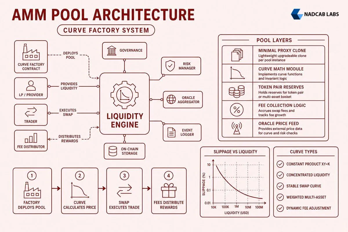
AMM curve design forms the mathematical backbone of decentralized exchange protocols, defining how asset prices adjust with each trade and how liquidity providers earn fees while managing risk. Pool factory patterns enable protocols to deploy customizable liquidity pools at scale, supporting diverse trading pairs and curve types without rewriting core infrastructure. Together, these architectural elements determine capital efficiency, slippage characteristics, and the economic viability of automated market makers in production DeFi systems.
Key Takeaways
- Constant product curves (x·y=k) provide simplicity but sacrifice capital efficiency; concentrated liquidity and stable swap curves optimize for specific asset classes
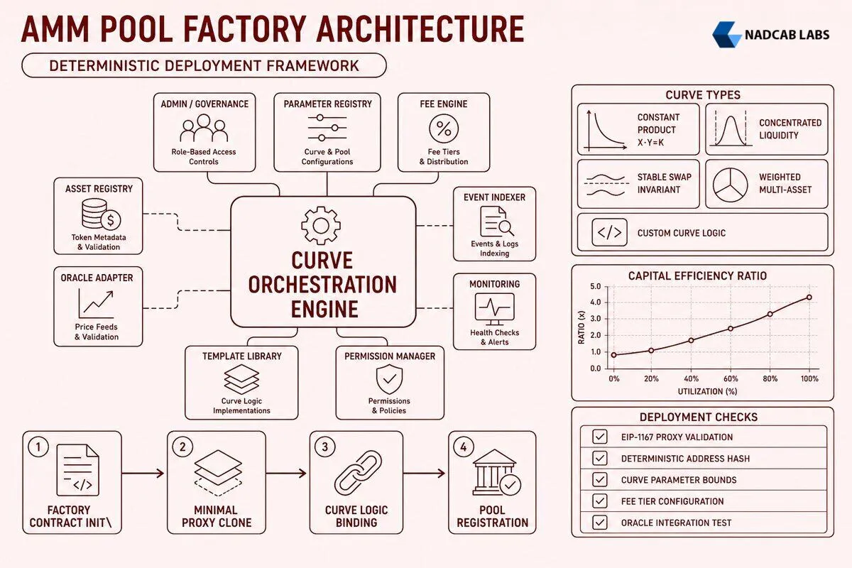
- Pool factory contracts use minimal proxy patterns (EIP-1167) and deterministic addressing to deploy thousands of customizable pools with minimal gas overhead
- Multi-asset pools employ weighted mathematics and amplification coefficients to reduce slippage and enable complex trading strategies
- Architecture-level impermanent loss mitigation combines tick spacing, dynamic fees, and embedded TWAP oracles to minimize LVR and MEV extraction
- Invariant testing and formal verification ensure curve integrity under extreme market conditions and prevent value-draining exploits
- Modular pool factory patterns support protocol upgrades via beacon proxies without requiring costly liquidity migrations
What Are the Core Mathematical Models Behind AMM Curve Design?
The constant product formula x·y=k represents the simplest and most battle-tested AMM curve design. When a trader swaps token X for token Y, the product of reserves must remain constant (ignoring fees). If a pool holds 100 ETH and 200,000 USDC, k equals 20,000,000. A swap that removes 10 ETH must add enough USDC to maintain the invariant, resulting in roughly 22,222 USDC deposited (before fees). This curve creates exponential price impact: larger trades face disproportionately worse execution prices because the formula forces the price to move along a hyperbola.
The constant product model excels in simplicity and robustness but wastes capital. Most liquidity sits far from the current market price, earning no fees. A pool with $10 million in TVL might only utilize $500,000 for trades within ±10% of spot price. This inefficiency motivated the development of alternative curves. Stable swap curves, pioneered by Curve Finance, use a hybrid invariant that behaves like a constant sum formula (x+y=k) near equilibrium and transitions to constant product behavior at extremes. The amplification coefficient A controls this transition: higher A values flatten the curve, reducing slippage for pegged assets like USDC-USDT but increasing divergence risk if the peg breaks.
The stable swap invariant takes the form: An^n Σx_i + D = ADn^n + D^(n+1)/(n^n Πx_i), where D represents the total value locked, n is the number of tokens, and A is the amplification parameter. For a two-asset pool with A=100, swapping 1% of reserves incurs roughly 0.01% price impact, compared to 1% impact in a constant product pool. This 100x improvement in capital efficiency makes stable swap curves ideal for correlated pairs but dangerous for volatile assets where the peg assumption fails.
Concentrated liquidity architecture, introduced by Uniswap v3, allows liquidity providers to allocate capital within custom price ranges. Instead of spreading liquidity across the entire price curve (0 to infinity), LPs deposit funds between a lower tick and upper tick. The pool contract divides the price space into discrete ticks (typically 0.01% or 0.1% spacing) and tracks liquidity density at each tick. When the market price crosses a tick boundary, the pool activates or deactivates the liquidity at that level. An LP providing liquidity between $1,800 and $2,200 for ETH/USDC earns fees only when the price trades in that range, but their capital is 5-10x more efficient than full-range liquidity at the same depth.
The mathematics of concentrated liquidity builds on the constant product formula but applies it piecewise. Within a single tick range, the curve follows x·y=k with virtual reserves that shift as the price moves. The effective liquidity L at the current price determines slippage: Δy = ΔL·Δ(√P), where P is the price. Tighter ranges concentrate L, reducing slippage per dollar of TVL but increasing the risk of price moving outside the range and leaving the LP with 100% exposure to the depreciating asset. This trade-off between capital efficiency and impermanent loss defines the core economic challenge in concentrated liquidity design.
| Curve Type | Capital Efficiency | Slippage (1% Swap) | Best Use Case | IL Risk |
|---|---|---|---|---|
| Constant Product | 1x (baseline) | ~1.0% | Volatile pairs (ETH/BTC) | Moderate |
| Stable Swap (A=100) | 50-100x | ~0.01% | Pegged assets (USDC/DAI) | Low (if peg holds) |
| Concentrated (±10% range) | 5-10x | ~0.2% | Narrow-range pairs (ETH/stETH) | High (range exit risk) |
| Weighted (80/20) | 2-3x | ~0.5% | Index funds (DeFi basket) | Moderate-Low |
Hybrid curve designs combine elements from multiple models to optimize for specific market conditions. Balancer’s weighted pools use the constant mean formula (x_1^w_1 · x_2^w_2 · … · x_n^w_n = k), where weights w_i sum to 1. An 80/20 ETH/USDC pool holds 80% of value in ETH and 20% in USDC, reducing impermanent loss compared to a 50/50 pool while maintaining liquidity. Dynamic weight adjustment mechanisms allow pools to rebalance automatically based on oracle prices or governance votes, creating synthetic exposure to portfolio rebalancing strategies without requiring active LP intervention.
How Do Pool Factory Patterns Enable Modular Liquidity Pool Deployment?
Pool factory contracts serve as the deployment engine for AMM protocols, allowing permissionless creation of new trading pairs without modifying core protocol code. The factory pattern separates pool logic (swap calculations, fee collection, liquidity management) from pool instantiation. A typical factory contract stores a template implementation address and uses the minimal proxy pattern (EIP-1167) to deploy lightweight clones. Each clone is a tiny bytecode wrapper (55 bytes) that delegates all calls to the implementation contract via DELEGATECALL, reducing deployment gas from ~3 million to ~100,000 per pool.
The factory contract generates deterministic pool addresses using CREATE2, which computes the address from the factory address, a salt (typically the hash of token addresses and fee tier), and the initialization code hash. This determinism enables off-chain address calculation before deployment and prevents duplicate pools for the same token pair and parameters. Uniswap v3’s factory uses CREATE2 with salt = keccak256(abi.encodePacked(token0, token1, fee)), ensuring that calling createPool(‘0xA0b…’, ‘0xC02…’, 3000) always produces the same pool address across all chains and deployment contexts.
Parameter customization at deployment allows each pool to specify fee tiers (0.01%, 0.05%, 0.3%, 1%), tick spacing (1, 10, 60, 200 basis points), and protocol fee switches. The factory contract validates parameters against whitelisted ranges to prevent economic attacks (e.g., 100% fees that would drain LPs). Some factory implementations support custom oracle integration, allowing pools to reference external price feeds for dynamic fee adjustment or circuit breakers. Governance hooks enable protocol-level fee collection: a portion of swap fees (e.g., 1/6th) can be redirected to a treasury address controlled by token holders, creating sustainable protocol revenue without taxing LPs directly.
Pool Factory Deployment Process
Choose tokens, fee tier, tick spacing
Compute CREATE2 address from salt
Deploy minimal proxy via factory
Set initial price, enable pool
Upgradeability strategies for pool logic present a fundamental tension: immutability builds trust, but bugs and efficiency improvements require updates. The beacon proxy pattern solves this by introducing an intermediate beacon contract that stores the current implementation address. All pool proxies query the beacon for the implementation address on each call. Upgrading the beacon updates all pools simultaneously without migrating liquidity or changing pool addresses. This pattern works well for non-contentious upgrades (gas optimizations, new view functions) but creates governance risk if the beacon controller is compromised or makes economically harmful changes.
The diamond pattern (EIP-2535) offers more granular upgradeability by splitting pool logic into multiple facets (swap facet, liquidity facet, oracle facet, etc.). Each facet is a separate contract, and the diamond proxy routes function calls to the appropriate facet based on a function selector mapping. Upgrading a single facet (e.g., replacing the swap algorithm) leaves other facets unchanged, reducing upgrade risk and gas costs. Balancer v2 uses a variant of this pattern with a Vault contract that holds all tokens and delegates swap logic to pool-specific contracts, enabling pool-level customization without fragmenting liquidity across isolated contracts.
Governance-controlled upgradeability typically requires a time-lock mechanism: proposed upgrades sit in a pending state for 24-72 hours before execution, giving LPs time to exit if they disagree with the change. Some protocols implement emergency pause functions that freeze swaps and liquidity changes in response to detected exploits, but these centralized controls conflict with the decentralization ethos. The trend in mature protocols is toward ossification: after initial development, the factory and pool logic become immutable, with new features deployed as separate pool types rather than upgrades to existing pools. This approach preserves trust while allowing innovation through opt-in migration to new pool versions.
What Smart Contract Structures Optimize Capital Efficiency in Multi-Asset Pools?
Weighted pool mathematics extends the constant product formula to support arbitrary token ratios and more than two assets. The Balancer weighted pool invariant is V = Π(B_i^W_i), where B_i is the balance of token i, W_i is its weight, and V is the pool’s invariant value. For a three-asset pool with weights 50% ETH, 30% WBTC, 20% LINK, the invariant is (B_ETH^0.5)(B_WBTC^0.3)(B_LINK^0.2) = V. Swapping ETH for WBTC changes both balances but preserves V (after accounting for fees). This formula allows LPs to create custom index funds: a DeFi basket pool might hold 40% UNI, 30% AAVE, 20% COMP, 10% SNX, automatically rebalancing as traders arbitrage price changes.
Dynamic weight adjustment mechanisms enable pools to shift allocations over time without requiring LPs to manually rebalance. A liquidity bootstrapping pool (LBP) might start with weights 95% ProjectToken / 5% USDC and gradually shift to 50/50 over 72 hours, creating continuous selling pressure that discovers a fair market price while preventing front-running bots from buying the entire supply at launch. The weight adjustment happens smoothly: at each block, the contract interpolates between start weights and end weights based on elapsed time. Traders arbitrage the changing weights, effectively performing a slow Dutch auction that distributes tokens widely while raising capital for the project.
Nested pool composition allows pools to hold LP tokens from other pools as assets, creating multi-layer index structures. A “DeFi Top 10” pool might hold LP tokens from ETH/USDC, WBTC/USDC, and UNI/USDC pools rather than holding the underlying tokens directly. This structure provides exposure to the top assets while earning swap fees from both the nested pools and the parent pool. The challenge is calculating accurate prices: the parent pool must query the nested pools for their spot prices and apply the weighted formula recursively. This introduces oracle dependencies and potential manipulation vectors if nested pools have low liquidity or can be flash-loan attacked.
Virtual reserves and amplification coefficients reduce slippage without requiring proportionally deeper liquidity. A stable swap pool with $10 million in actual reserves might behave like a $500 million constant product pool near equilibrium by using virtual reserves: x_virtual = x_actual + offset. The offset shifts the curve’s center, flattening the price impact region. The amplification coefficient A in stable swap curves serves a similar purpose: it interpolates between constant sum (A=∞, zero slippage, infinite divergence risk) and constant product (A=0, high slippage, bounded divergence). Tuning A requires balancing capital efficiency against the risk that correlated assets depeg and drain the pool through arbitrage.
The relationship between amplification and slippage follows: slippage ≈ (trade_size / liquidity) / A for small trades in stable swap pools. A pool with A=100 and $10 million liquidity incurs roughly 0.01% slippage on a $100,000 trade, compared to 1% slippage in a constant product pool with the same liquidity. However, if one asset depegs by 5%, the amplified curve creates arbitrage opportunities that can drain the pool’s holdings of the pegged asset. The 2020 mUSD depeg incident demonstrated this risk: Curve pools with high A values lost significant value as arbitrageurs swapped depegged mUSD for USDC at near-1:1 rates until the pools held mostly worthless mUSD.
Capital Efficiency Comparison by Pool Type
Multi-asset pools face additional complexity in fee distribution and liquidity accounting. In a two-asset pool, all swaps move along a single price curve, but a four-asset pool supports six trading pairs (A/B, A/C, A/D, B/C, B/D, C/D). Each swap affects all four balances through the weighted invariant, and fees must be allocated proportionally to the liquidity that facilitated the trade. The smart contract must track cumulative fees per token and distribute them to LPs based on their share of total liquidity at the time of each swap. This accounting overhead increases gas costs: a Balancer v2 swap costs roughly 120,000 gas compared to 80,000 for a Uniswap v2 swap, with the difference primarily in fee calculation and multi-token balance updates.
Protocols building DeFi Development solutions often implement custom pool types to optimize for specific use cases. A real estate tokenization platform might use a weighted pool with 70% property tokens and 30% stablecoins to provide liquidity while minimizing impermanent loss for long-term holders. A prediction market might use a constant sum curve (x+y=k) for binary outcome tokens, ensuring 1:1 swaps until one outcome resolves. These specialized curves require careful mathematical analysis to ensure they preserve value and cannot be exploited through adversarial trading sequences or flash loan attacks.
How Can Architecture-Level Design Mitigate Impermanent Loss and MEV Risks?
Loss-versus-rebalancing (LVR) represents the fundamental arbitrage tax that LPs pay to keep pool prices aligned with external markets. When the market price of ETH rises from $2,000 to $2,100, arbitrageurs buy ETH from the pool at the stale price and sell it on centralized exchanges at the new price, extracting value from LPs. The magnitude of LVR depends on price volatility, block time, and pool fee tier. Research shows that LPs in volatile pairs lose roughly 5-10% annually to LVR even in efficient markets, often exceeding fee income. Architectural mitigations include increasing tick spacing (forcing larger price jumps between rebalances), implementing dynamic fees that rise with volatility, and using time-weighted average price (TWAP) oracles to delay price updates until arbitrage becomes unprofitable.
Tick spacing in concentrated liquidity pools controls the granularity of price movement and rebalancing frequency. Uniswap v3 offers tick spacings of 1, 10, 60, and 200 basis points, corresponding to fee tiers of 0.01%, 0.05%, 0.3%, and 1%. Wider tick spacing reduces LVR by forcing arbitrageurs to wait for larger price moves before trading becomes profitable, but it also increases slippage for retail traders. A 200-basis-point tick spacing means the pool price can only update in 2% increments, so a 1% market move produces no arbitrage opportunity. However, a trader swapping $10,000 in this pool faces higher slippage than in a 10-basis-point pool because liquidity is concentrated in fewer, wider ticks. The optimal tick spacing balances LVR reduction against user experience degradation.
Dynamic fee mechanisms adjust swap fees in real-time based on market conditions. A pool might charge 0.05% fees during calm periods and automatically increase to 0.3% when volatility spikes, capturing more value from arbitrageurs while remaining competitive for normal trades. The challenge is designing a fee update mechanism that cannot be manipulated: if fees depend on recent price volatility, an attacker could artificially inflate volatility through wash trading to force fee increases, then profit from the wider spread. Robust dynamic fee implementations use exponential moving averages of squared price changes over multiple blocks and cap fee adjustments to prevent sudden jumps that would fragment liquidity across pools with different fee tiers.
Time-weighted average price oracles embedded in pool contracts reduce the arbitrage attack surface by making it expensive to manipulate the pool’s reported price. Instead of using the instantaneous spot price (which can be manipulated within a single block via flash loans), TWAP oracles accumulate price observations over time and report the average. Uniswap v2 and v3 pools maintain cumulative price variables that increase by the spot price at each block: price_cumulative += spot_price * time_elapsed. External contracts can query price_cumulative at two different timestamps and divide by the elapsed time to get a manipulation-resistant average price. An attacker would need to sustain a manipulated price for the entire TWAP window (typically 10-30 minutes) to influence the oracle, making attacks prohibitively expensive in liquid pools.
| Mitigation Technique | LVR Reduction | Trade-off | Implementation Complexity |
|---|---|---|---|
| Wide Tick Spacing (200bp) | 40-60% reduction | Higher slippage for users | Low (parameter change) |
| Dynamic Fees (volatility-based) | 30-50% reduction | Complexity, manipulation risk | High (oracle integration) |
| TWAP Oracle Integration | 20-30% reduction | Stale prices, delayed updates | Medium (storage overhead) |
| Batch Auctions (commit-reveal) | 60-80% reduction | Delayed execution, UX friction | Very High (protocol redesign) |
Batch auction mechanisms prevent front-running and sandwich attacks by collecting all swap requests during a time window (e.g., 12 seconds) and executing them simultaneously at a uniform clearing price. Traders submit orders during the commit phase, and the protocol computes the price that balances supply and demand during the reveal phase. This eliminates the concept of transaction ordering within a batch: there is no “first” or “last” trade to sandwich. CoW Swap and Gnosis Protocol use batch auctions to protect users from MEV extraction, achieving 60-80% reduction in effective slippage compared to traditional AMMs. The trade-off is execution latency: users must wait for the batch to close and clear before their trades settle, which conflicts with the instant-swap UX that made AMMs popular.
Commit-reveal schemes add a cryptographic layer to batch auctions by requiring traders to submit hashed orders during the commit phase and reveal the plaintext orders only after the commit window closes. This prevents validators and searchers from observing pending orders and front-running them, because the order details are encrypted until all commits are finalized. The reveal phase validates that each revealed order matches its committed hash and then executes the batch. This approach is highly resistant to MEV but adds significant complexity: users must submit two transactions per trade, and the protocol must handle cases where users commit but fail to reveal (either due to network issues or intentional griefing).
Protocols implementing liquidity pool integration for market makers often combine multiple mitigation techniques. A professional market-making firm providing liquidity to a volatile pair might use concentrated liquidity with wide tick spacing, dynamic fees tied to realized volatility, and TWAP-based rebalancing triggers to minimize LVR while maintaining competitive quotes. The firm’s smart contracts monitor the pool’s TWAP oracle and automatically shift liquidity ranges when the 30-minute average price deviates more than 2% from the current range center, reducing the window for arbitrageurs to extract value before the LP adapts.
What Are the Best Practices for Auditing and Testing Liquidity Pool Smart Contracts?
Invariant testing validates that core mathematical properties hold under all possible sequences of operations. For a constant product pool, the invariant x·y≥k must hold after every swap (the ≥ accounts for fees increasing k over time). A comprehensive invariant test suite generates thousands of randomized swap sequences, checking that k never decreases and that the pool cannot be drained through any combination of trades. Echidna and Foundry’s invariant testing frameworks excel at this: they mutate input parameters (swap amounts, token addresses, fee tiers) and execute operations in random orders, searching for sequences that violate the invariant. A typical test might run 10,000 iterations with random swap sizes from 0.001% to 50% of reserves, verifying that reserves never go negative and that LP shares always represent proportional ownership.
Formal verification of mathematical properties uses symbolic execution and theorem provers to mathematically prove that certain bugs cannot exist. For example, a formal verification tool can prove that no sequence of swaps and liquidity operations in a Uniswap v3 pool can result in more tokens being withdrawn than were deposited (conservation of value). The tool models the smart contract as a set of mathematical constraints and searches for counterexamples: input sequences that violate the property. If no counterexample exists after exhaustive search, the property is proven. Certora and Runtime Verification provide formal verification services for DeFi protocols, catching subtle bugs that traditional testing misses, such as rounding errors that accumulate over millions of transactions or edge cases in concentrated liquidity tick transitions.
Edge-case liquidity scenarios test pool behavior under extreme conditions: single-sided deposits, full-range exits, price movements that cross multiple tick boundaries in one transaction, and swaps that consume 99.9% of reserves. A robust test suite includes cases like: (1) LP deposits $1 million, price moves 50%, LP withdraws — verify impermanent loss calculation matches theory. (2) 100 LPs deposit random amounts in random ranges, 10,000 swaps occur, all LPs withdraw — verify sum of withdrawals equals initial deposits plus fees minus gas. (3) Pool has $100 in liquidity, attacker attempts a $1 billion swap — verify transaction reverts with appropriate error message rather than causing integer overflow or unexpected state changes.
Gas optimization patterns specific to AMM contracts include storage packing (storing multiple variables in a single storage slot to reduce SLOAD costs), unchecked arithmetic (using unchecked blocks for calculations that cannot overflow, saving ~3 gas per operation), and batch operations (allowing multiple swaps or liquidity changes in a single transaction to amortize base gas costs). A well-optimized swap function might pack token balances, fee accumulators, and last-update timestamps into two storage slots instead of four, reducing gas by ~4,000 per swap. However, aggressive optimization introduces risk: unchecked arithmetic can cause silent overflows if assumptions about input ranges are violated, and storage packing can make the code harder to audit and maintain.
Smart Contract Audit Checklist for AMM Pools
Reentrancy guards specific to swap and liquidity operations prevent attackers from re-entering the pool contract during a callback and manipulating state. The classic reentrancy pattern uses a mutex lock: set locked=true at function entry, revert if already locked, execute logic, set locked=false before return. However, this pattern adds ~5,000 gas per call due to storage writes. Modern AMM implementations use the checks-effects-interactions (CEI) pattern: perform all state updates before making external calls (token transfers). Since the pool’s internal state (balances, fee accumulators) is updated before transferring tokens, even if the token contract re-enters the pool, it sees the post-swap state and cannot extract additional value. This pattern eliminates the need for explicit locks in most cases, saving gas while maintaining security.
Protocols developing token vesting smart contract architecture or similar time-dependent mechanisms must carefully test interaction between vesting schedules and AMM liquidity. For example, if vested tokens can be deposited as AMM liquidity, the contract must handle cases where the vesting cliff passes while tokens are locked in a pool, or where a user tries to withdraw liquidity that includes unvested tokens. The audit must verify that vesting restrictions cannot be bypassed through AMM operations and that liquidity withdrawals correctly split vested and unvested portions.
Integration testing with real-world protocols validates that the AMM contract behaves correctly when composed with other DeFi primitives. A comprehensive test suite includes: (1) Flash loan attacks: borrow $10 million from Aave, manipulate the pool, repay loan — verify no value extraction. (2) Oracle manipulation: use the pool as a price oracle for a lending protocol, attempt to liquidate positions via price manipulation — verify TWAP prevents exploitation. (3) Cross-chain scenarios: for protocols supporting multi-chain MLM smart contract architecture, test that liquidity remains consistent across bridges and that cross-chain arbitrage cannot drain pools. These integration tests catch issues that unit tests miss, such as unexpected interactions between AMM math and external protocol assumptions.
Continuous monitoring and incident response procedures are essential post-deployment. Leading AMM protocols run monitoring bots that track invariant violations, unusual trading patterns (e.g., swaps that move price >10% in one transaction), and oracle deviations. If a bot detects an anomaly, it triggers alerts to the security team and can automatically pause the pool if thresholds are exceeded. The Blockchain archive node infrastructure enables post-incident analysis: replaying historical transactions to understand exploit mechanics and verify that fixes prevent recurrence. Protocols should maintain runbooks for common incident types (oracle failure, bridge hack, flash loan attack) with pre-approved response procedures to minimize response time during active exploits.
Developers building systems similar to HIPAA compliant blockchain architecture or RPA architecture design patterns can apply similar rigor to AMM audits: define formal invariants, test exhaustively, and implement defense-in-depth with multiple layers of protection (circuit breakers, rate limits, anomaly detection). The financial stakes in AMM protocols (billions in TVL) justify the investment in formal methods and continuous security monitoring that would be overkill for lower-value applications.
AMM curve design and pool factory patterns represent the architectural foundation of decentralized exchange infrastructure. The mathematical elegance of constant product curves enabled the first wave of DeFi adoption, while concentrated liquidity and stable swap innovations pushed capital efficiency to levels competitive with centralized exchanges. Pool factory contracts democratized liquidity deployment, allowing anyone to create custom trading pairs without permission or technical expertise. As the ecosystem matures, the focus shifts from inventing new curve types to hardening existing designs against MEV extraction, impermanent loss, and smart contract vulnerabilities. Projects building real estate token liquidity pool mechanics or other novel use cases inherit these battle-tested patterns, adapting them to domain-specific requirements while maintaining the core principles of trustless, permissionless exchange.
Frequently Asked Questions
Q1.What is the difference between constant product and concentrated liquidity curves in AMM design?
Constant product curves (x*y=k) distribute liquidity evenly across all price ranges, suitable for volatile pairs but capital-inefficient. Concentrated liquidity curves allow LPs to allocate capital within specific price ranges, achieving 100-4000x capital efficiency for stable or correlated assets. Uniswap V2 uses constant product; V3 implements concentrated liquidity with customizable tick ranges, enabling higher fee generation per dollar locked but requiring active position management.
Q2.How do pool factory contracts enable permissionless liquidity pool creation?
Pool factory contracts use the CREATE2 opcode to deterministically deploy new pool instances at predictable addresses based on token pair hashes. Anyone can call the factory’s createPool function with token addresses and fee tier parameters. The factory maintains a registry mapping token pairs to pool addresses, enforces single-pool-per-pair rules, and clones a minimal proxy implementation to reduce deployment gas costs from ~3M to ~200k gas per pool.
Q3.What are the key smart contract components of a multi-asset liquidity pool?
Core components include: token balance tracking arrays, invariant calculation functions (curve logic), swap routing with slippage checks, liquidity deposit/withdrawal handlers, LP token minting/burning mechanisms, fee accrual accounting per token, oracle price accumulator updates, and reentrancy guards. Advanced pools add amplification coefficients for stableswaps, dynamic fee adjustment based on volatility, and multi-hop routing optimization to minimize price impact across asset combinations.
Q4.How can liquidity pool architecture reduce impermanent loss at the code level?
Architectural strategies include: implementing dynamic fee structures that increase during high volatility to compensate LPs, using bonding curves with lower curvature (StableSwap A parameter) for correlated assets, adding single-sided liquidity options with synthetic counterparties, incorporating price oracle checks to pause swaps during manipulation attempts, and designing asymmetric rebalancing mechanisms that favor the appreciating asset. Some protocols implement loss-protection vaults that socialize IL across longer timeframes.
Q5.What security vulnerabilities are unique to AMM curve implementations?
Critical vulnerabilities include: precision loss in fixed-point math causing rounding exploits, reentrancy attacks during multi-token swaps, price oracle manipulation via flash loans affecting curve parameters, integer overflow in exponential bonding curves, sandwich attacks exploiting predictable slippage, and donation attacks that corrupt invariant calculations. Curve-specific risks involve amplification parameter misconfiguration enabling drainage and tick manipulation in concentrated liquidity allowing JIT liquidity extraction.
Q6.How do modular pool factory patterns support protocol upgrades without liquidity migration?
Modular factories separate pool logic into upgradeable libraries called via delegatecall, allowing core math updates without touching liquidity storage. Proxy patterns (UUPS, transparent, beacon) enable logic contract replacement while preserving state. Factory registries can deprecate old implementations and route new swaps to upgraded pools. Some designs use adapter contracts that translate between pool versions, letting liquidity remain in original pools while new features deploy separately, avoiding the capital inefficiency of forced migrations.
Explore Services
Related Services
Reviewed by

Naman Singh
Co-Founder & CEO, Nadcab Labs
Naman Singh is the Co-Founder and CEO of Nadcab Labs, where he drives the company’s vision, global growth, and strategic expansion in blockchain, fintech, and digital transformation. A serial entrepreneur, Naman brings deep hands-on experience in building, scaling, and commercializing technology-driven businesses. At Nadcab Labs, Naman works closely with enterprises, governments, and startups to design and implement secure, scalable, and business-ready Web3 and blockchain solutions. He specializes in transforming complex ideas into high-impact digital products aligned with real business objectives. Naman has led the development of end-to-end blockchain ecosystems, including token creation, smart contracts, DeFi and NFT platforms, payment infrastructures, and decentralized applications. His expertise extends to tokenomics design, regulatory alignment, compliance strategy, and go-to-market planning—helping projects become investor-ready and built for long-term sustainability. With a strong focus on real-world adoption, Naman believes in building blockchain solutions that deliver measurable value, solve practical problems, and unlock new growth opportunities for organizations worldwide.